WbW-Pro function documentation
Each of the following functions are methods of WbEnvironment class. Tools may be called using the convention in the following example:
from whitebox_workflows import WbEnvironment

wbe = WbEnvironment()
# Set up the environment, e.g. working directory, verbose mode, num_procs
raster = wbe.read_raster('my_raster.tif') # Read some kind of data
result = wbe.shape_index(raster) # Call some kind of function
...
- accumulation_curvature
- assess_route
- average_horizon_distance
- breakline_mapping
- canny_edge_detection
- classify_lidar
- colourize_based_on_class
- colourize_based_on_point_returns
- curvedness
- dbscan
- dem_void_filling
- depth_to_water
- difference_curvature
- evaluate_training_sites
- filter_lidar
- filter_lidar_by_percentile
- filter_lidar_by_reference_surface
- fix_dangling_arcs
- fuzzy_knn_classification
- generalize_classified_raster
- generalize_with_similarity
- generating_function
- horizon_area
- horizontal_excess_curvature
- hydrologic_connectivity
- image_segmentation
- image_slider
- improved_ground_point_filter
- inverse_pca
- knn_classification
- knn_regression
- lidar_contour
- lidar_eigenvalue_features
- lidar_point_return_analysis
- lidar_sibson_interpolation
- local_hypsometric_analysis
- logistic_regression
- low_points_on_headwater_divides
- min_dist_classification
- minimal_dispersion_flow_algorithm
- modify_lidar
- multiscale_curvatures
- nibble
- openness
- parallelepiped_classification
- phi_coefficient
- piecewise_contrast_stretch
- prune_vector_streams
- random_forest_classification_fit
- random_forest_classification_predict
- random_forest_regression_fit
- random_forest_regression_predict
- reconcile_multiple_headers
- recover_flightline_info
- recreate_pass_lines
- remove_field_edge_points
- remove_raster_polygon_holes
- ridge_and_valley_vectors
- ring_curvature
- river_centerlines
- rotor
- shadow_animation
- shadow_image
- shape_index
- sieve
- sky_view_factor
- skyline_analysis
- slope_vs_aspect_plot
- smooth_vegetation_residual
- sort_lidar
- split_lidar
- svm_classification
- svm_regression
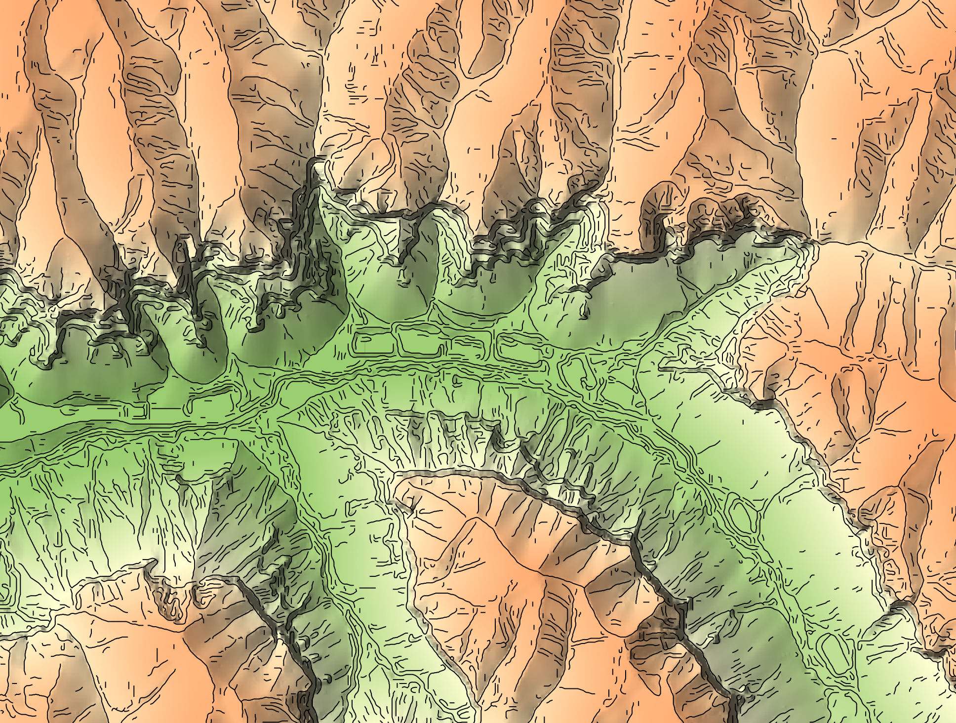
- topo_render
- topographic_position_animation
- topological_breach_burn
- unsphericity
- vertical_excess_curvature
- yield_filter
- yield_map
- yield_normalization
accumulation_curvature
License Information
Use of this function requires a license for Whitebox Workflows for Python Professional (WbW-Pro). Please visit www.whiteboxgeo.com to purchase a license.
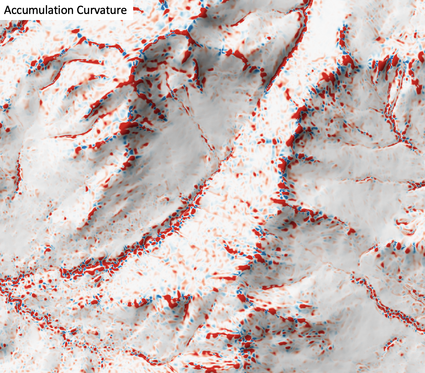
Description
This tool calculates the accumulation curvature from a digital elevation model (DEM). Accumulation curvature is the product of profile (vertical) and tangential (horizontal) curvatures at a location (Shary, 1995). This variable has positive values, zero or greater. Florinsky (2017) states that accumulation curvature is a measure of the extent of local accumulation of flows at a given point in the topographic surface. Accumulation curvature is measured in units of m-2.
The user must specify the name of the input DEM (dem) and the output raster (output). The
The Z conversion factor (zfactor) is only important when the vertical and horizontal units are not the
same in the DEM. When this is the case, the algorithm will multiply each elevation in the DEM by the
Z Conversion Factor. Curvature values are often very small and as such the user may opt to log-transform
the output raster (log). Transforming the values applies the equation by Shary et al. (2002):
Θ' = sign(Θ) ln(1 + 10n|Θ|)
where Θ is the parameter value and n is dependent on the grid cell size.
For DEMs in projected coordinate systems, the tool uses the 3rd-order bivariate Taylor polynomial method described by Florinsky (2016). Based on a polynomial fit of the elevations within the 5x5 neighbourhood surrounding each cell, this method is considered more robust against outlier elevations (noise) than other methods. For DEMs in geographic coordinate systems (i.e. angular units), the tool uses the 3x3 polynomial fitting method for equal angle grids also described by Florinsky (2016).
References
Florinsky, I. (2016). Digital terrain analysis in soil science and geology. Academic Press.
Florinsky, I. V. (2017). An illustrated introduction to general geomorphometry. Progress in Physical Geography, 41(6), 723-752.
Shary PA (1995) Land surface in gravity points classification by a complete system of curvatures. Mathematical Geology 27: 373–390.
Shary P. A., Sharaya L. S. and Mitusov A. V. (2002) Fundamental quantitative methods of land surface analysis. Geoderma 107: 1–32.
See Also
tangential_curvature, profile_curvature, minimal_curvature, maximal_curvature, mean_curvature, gaussian_curvature
Function Signature
def accumulation_curvature(self, dem: Raster, log_transform: bool = False, z_factor: float = 1.0) -> Raster: ...
assess_route
License Information
Use of this function requires a license for Whitebox Workflows for Python Professional (WbW-Pro). Please visit www.whiteboxgeo.com to purchase a license.
Description
This tool assesses the variability in slope, elevation, and visibility along a line vector, which may
be a footpath, road, river or any other route. The user must specify the name of the input line vector
(routes), the input raster digital elevation model file (dem), and the output line vector
(output). The algorithm initially splits the input line vector in equal-length segments (length).
For each line segment, the tool then calculates the average slope (AVG_SLOPE), minimum and maximum
elevations (MIN_ELEV, MAX_ELEV), the elevation range or relief (RELIEF), the path sinuosity
(SINUOSITY), the number of changes in slope direction or breaks-in-slope (CHG_IN_SLP), and the
maximum visibility (VISIBILITY). Each of these metrics are output to the attribute table of the output
vector, along with the feature identifier (FID); any attributes associated with the input parent
feature will also be copied into the output table. Slope and elevation metrics are measured along the
2D path based on the elevations of each of the row and column intersection points of the raster with
the path, estimated from linear-interpolation using the two neighbouring elevations on either side of
the path. Sinuosity is calculated as the ratio of the along-surface (i.e. 3D) path length, divided by
the 3D distance between the start and end points of the segment. CHG_IN_SLP can be thought of as a crude
measure of path roughness, although this will be very sensitive to the quality of the DEM. The visibility
metric is based on the Yokoyama et al. (2002) openness index, which calculates the average horizon
angle in the eight cardal directions to a maximum search distance (dist), measured in grid cells.
Note that the input DEM must be in a projected coordinate system. The DEM and the input routes vector must be also share the same coordinate system. This tool also works best when the input DEM is of high quality and fine spatial resolution, such as those derived from LiDAR data sets.
Maximum segment visibility:
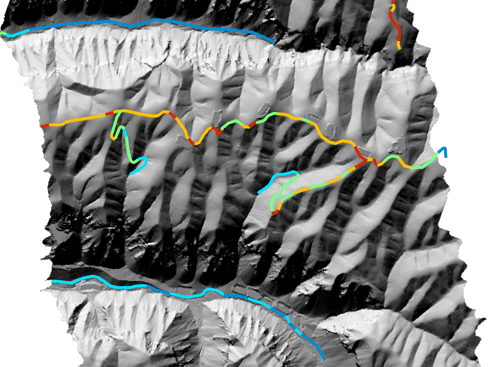
Average segment slope:
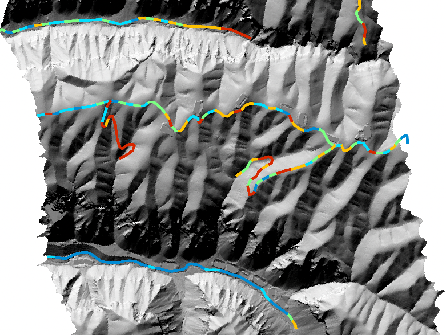
For more information about this tool, see this blog on the WhiteboxTools homepage.
See Also
Function Signature
def assess_route(self, routes: Vector, dem: Raster, segment_length: float = 100.0, search_radius: int = 15) -> Vector: ...
average_horizon_distance
License Information
Use of this function requires a license for Whitebox Workflows for Python Professional (WbW-Pro). Please visit www.whiteboxgeo.com to purchase a license.
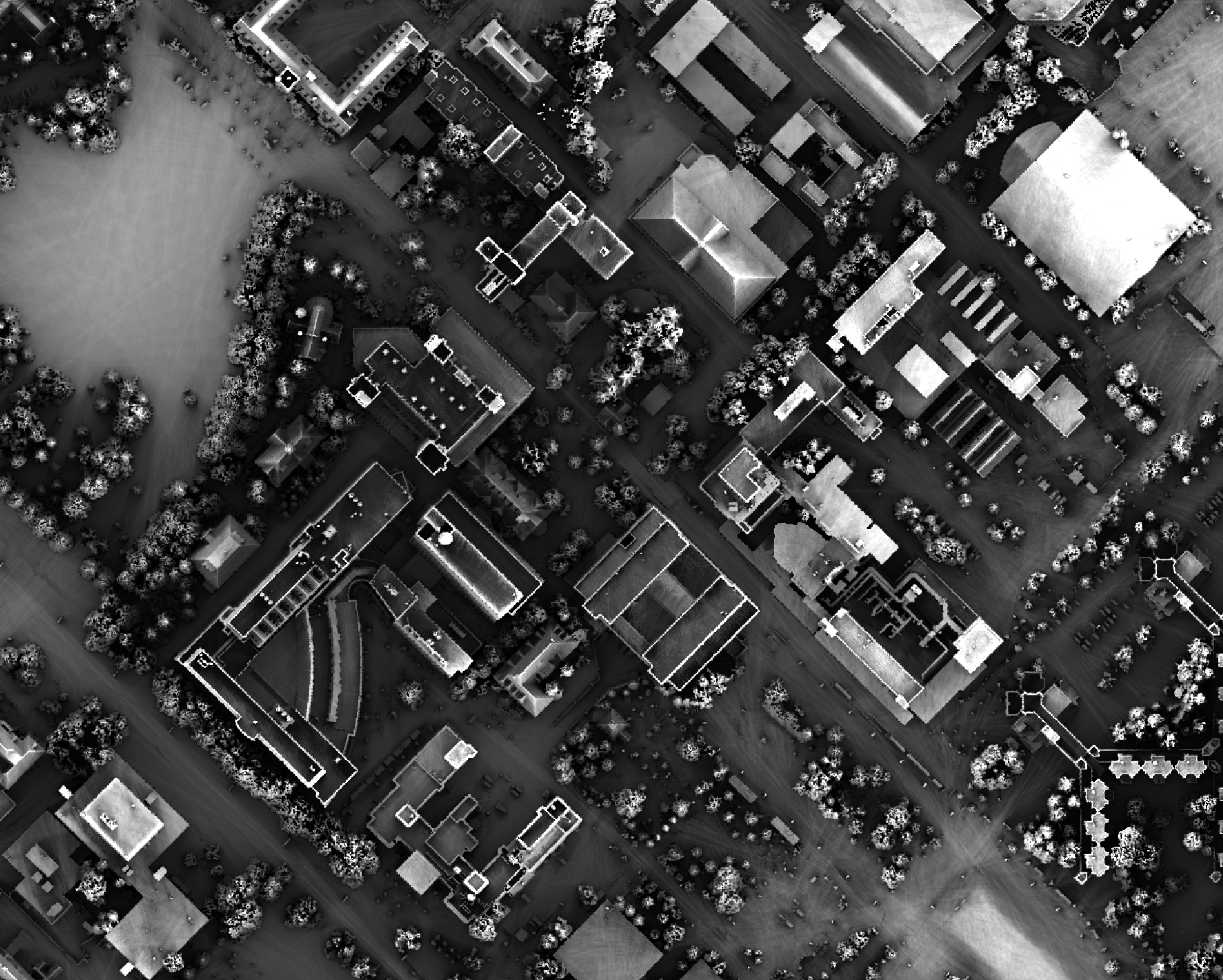
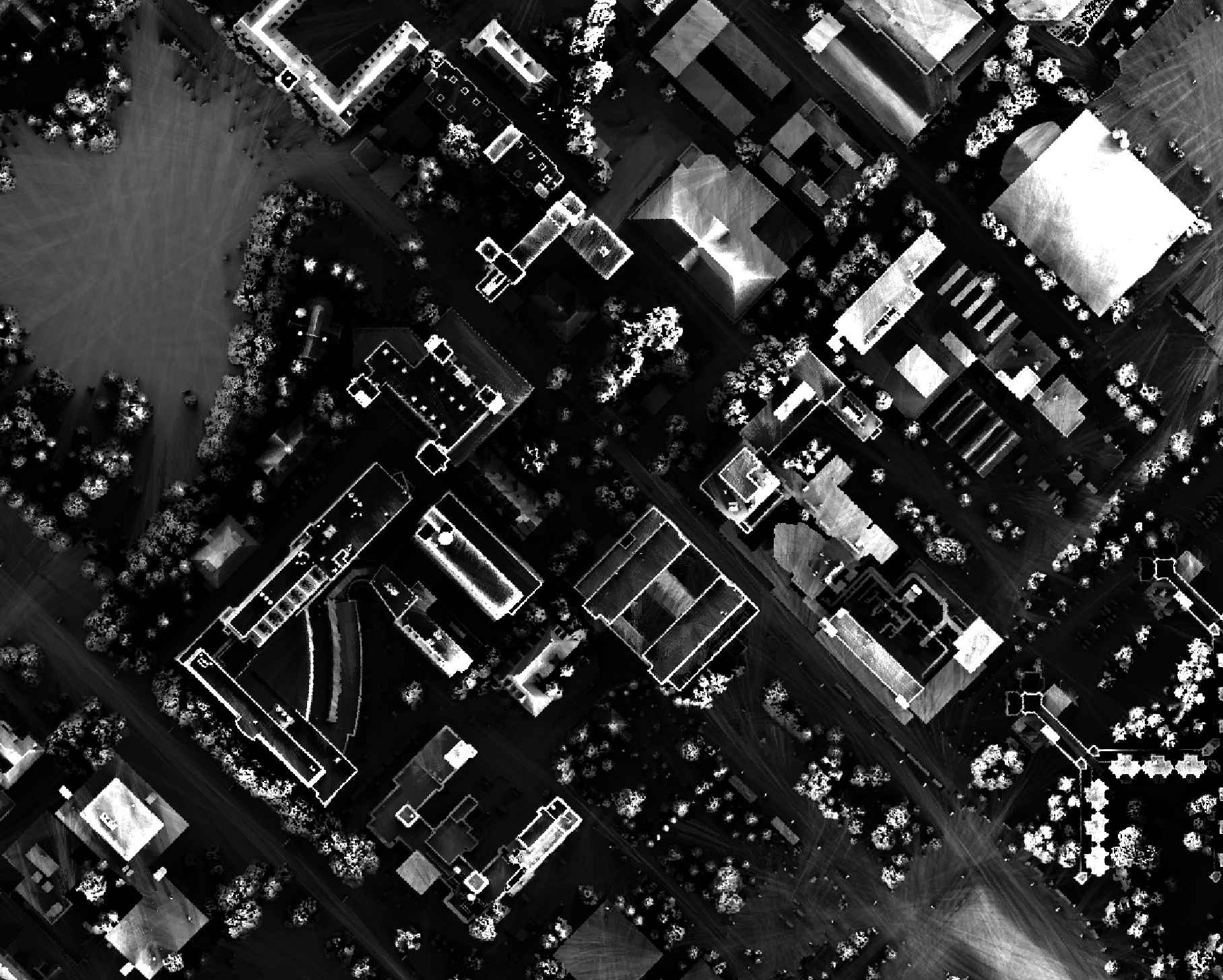
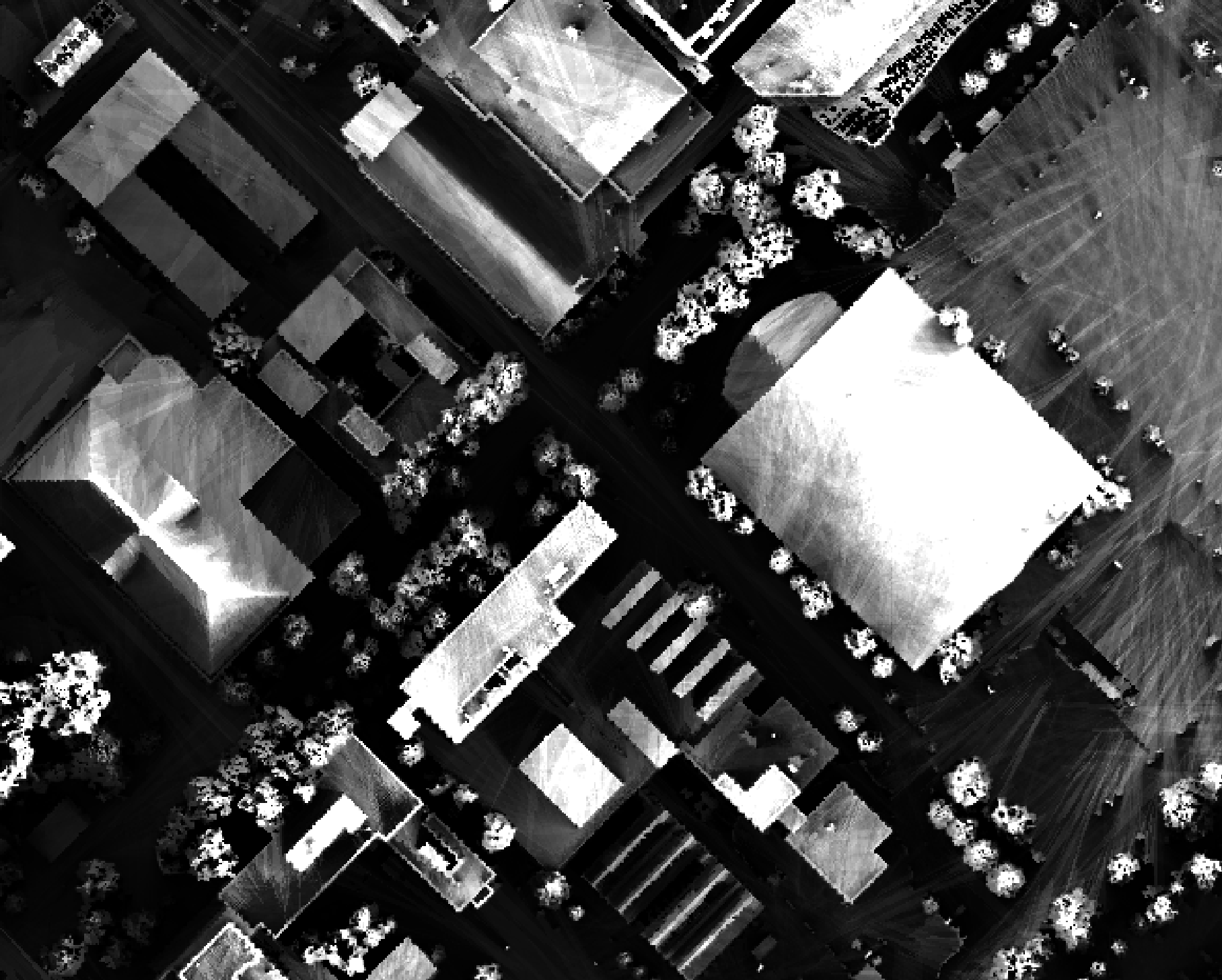
This tool calculates the spatial pattern of average distance to the horizon based on an input digital elevation model (DEM). As such, the index is a measure of landscape visibility. In the image below, lighter areas have a longer average distance to the horizon, measured in map units.
The user must specify an input DEM (dem), the azimuth fraction (az_fraction), the maximum search
distance (max_dist), and the height offset of the observer (observer_hgt_offset). The input DEM
should usually be a digital surface model (DSM) that contains significant off-terrain objects. Such a
model, for example, could be created using the first-return points of a LiDAR data set, or using the
lidar_digital_surface_model tool. The azimuth
fraction should be an even divisor of 360-degrees and must be between 1-45 degrees.
The tool operates by calculating horizon angle (see horizon_angle)
rasters from the DSM based on the user-specified azimuth fraction (az_fraction). For example, if an azimuth
fraction of 15-degrees is specified, horizon angle rasters would be calculated for the solar azimuths 0,
15, 30, 45... A horizon angle raster evaluates the vertical angle between each grid cell in a DSM and a
distant obstacle (e.g. a mountain ridge, building, tree, etc.) that obscures the view in a specified
direction. In calculating horizon angle, the user must specify the maximum search distance (max_dist),
in map units, beyond which the query for higher, more distant objects will cease. This parameter strongly
impacts the performance of the function, with larger values resulting in significantly longer processing-times.
The observer_hgt_offset parameter can be used to add an increment to the source cell's elevation. For
example, the following image shows the spatial pattern derived from a LiDAR DSM using observer_hgt_offset = 0.0:
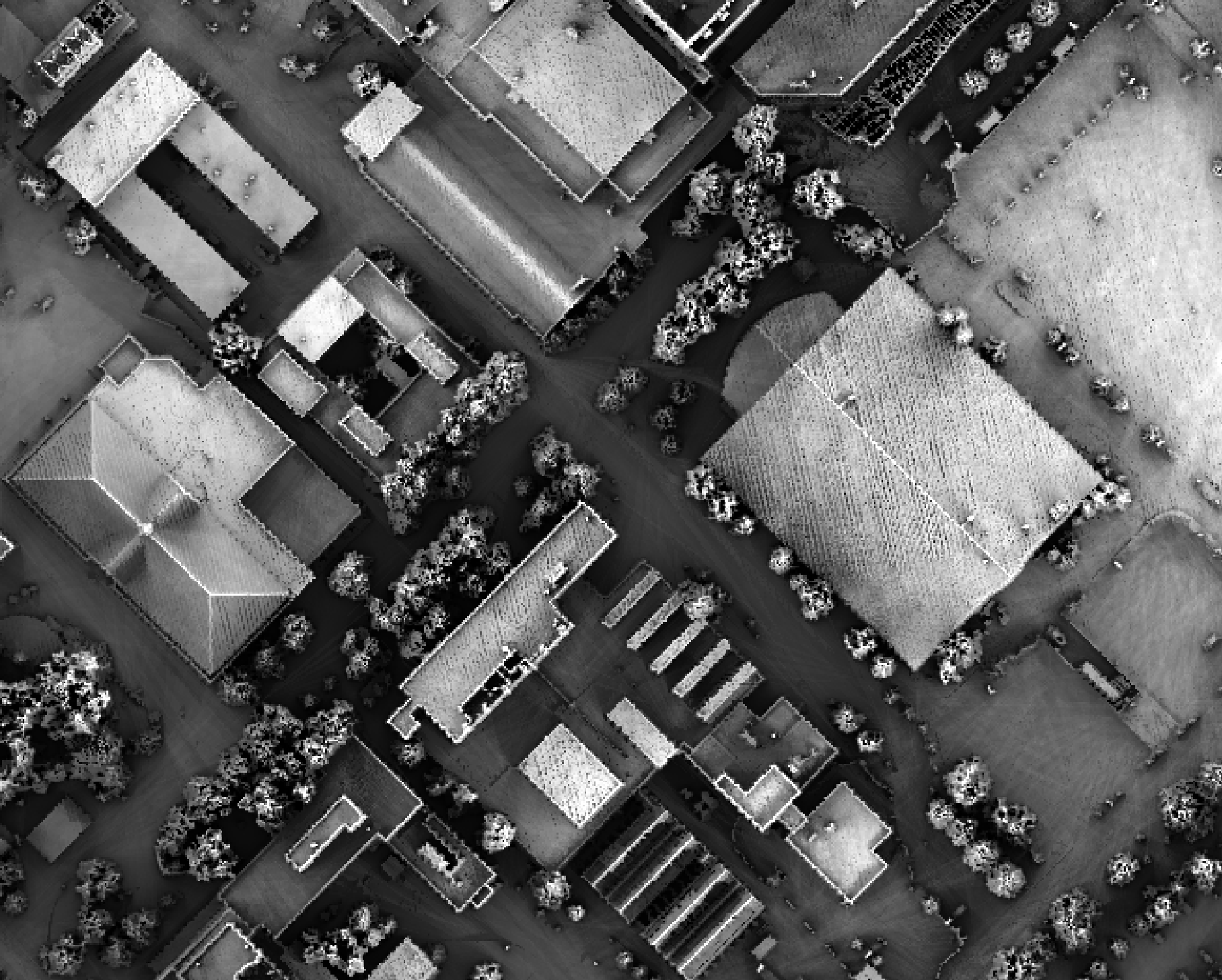
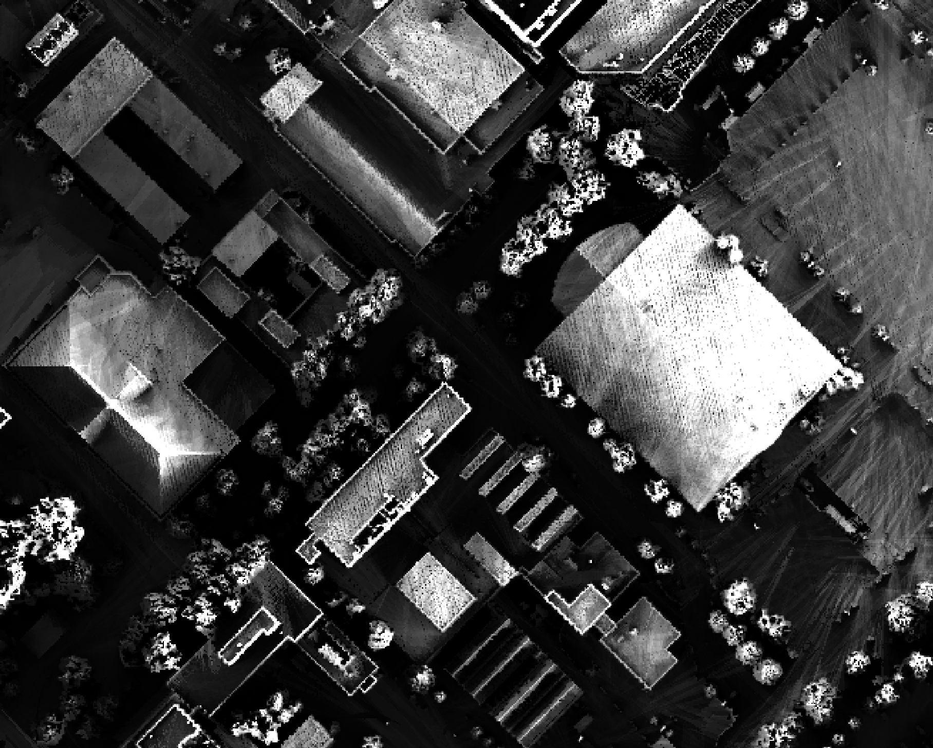
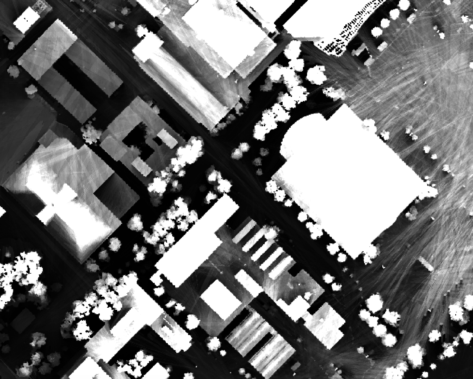
Notice that there are several places, plarticularly on the flatter rooftops, where the local noise in the LiDAR DEM, associated with the individual scan lines, has resulted in a noisy pattern in the output. By adding a small height offset of the scale of this noise variation (0.15 m), we see that most of this noisy pattern is removed in the output below:
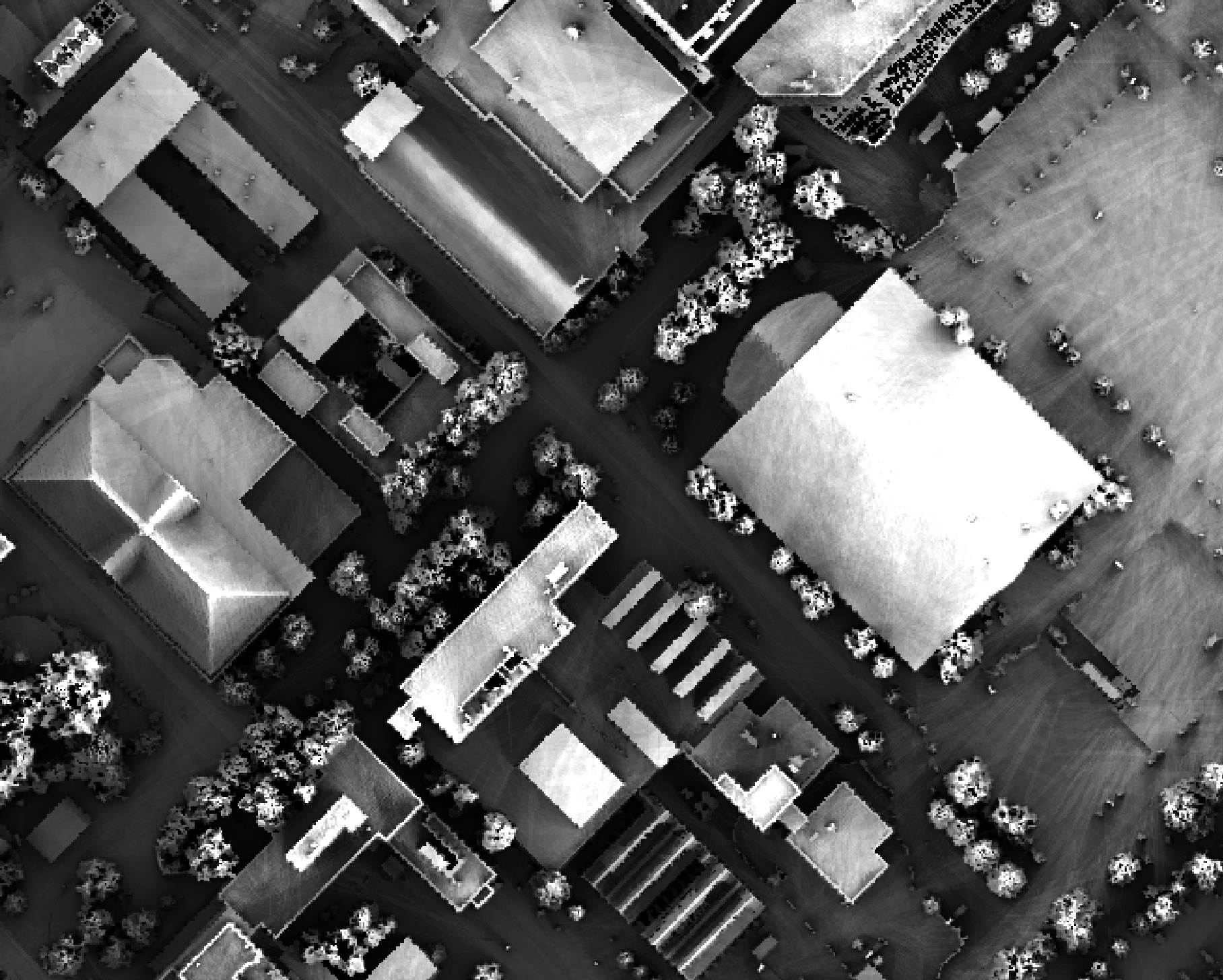
This feature makes the function more robust against DEM noise. As another example of the usefulness of
this additional parameter, in the image below, the observer_hgt_offset parameter has been used to
measure the pattern of the index at a typical human height (1.7 m):
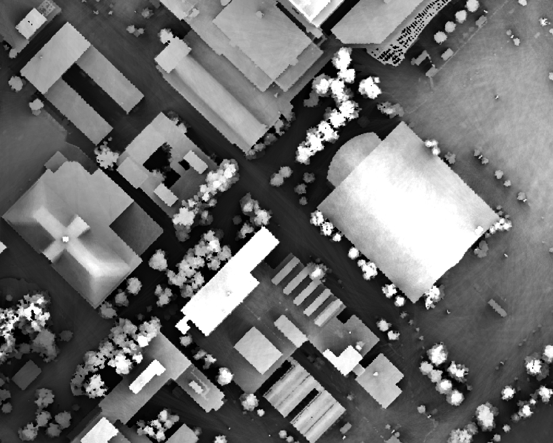
Notice how at this height the average horizon distance becomes much farther on some of the flat rooftops where a guard wall prevents further viewing areas at shorter observer heights.
The output of this function is similar to the Average View Distance provided by the Sky View tool in Saga GIS. However, for a given maximum search distance, the Whitebox tool is likely faster to compute and has the added advantage of offering the observer's height parameter, as described above.
See Also
sky_view_factor, horizon_area, openness, lidar_digital_surface_model, horizon_angle
Function Signature
def average_horizon_distance(self, dem: Raster, az_fraction: float = 5.0, max_dist: float = float('inf'), observer_hgt_offset: float = 0.0) -> Raster: ...
breakline_mapping
License Information
Use of this function requires a license for Whitebox Workflows for Python Professional (WbW-Pro). Please visit www.whiteboxgeo.com to purchase a license.
Description
This tool can be used to map breaklines in an input digital elevation model (DEM; input). Breaklines are
locations of high surface curvature, in any direction, measured using curvedness. Curvedness values are
log-transformed using the resolution-dependent method proposed by Shary et al. (2002). Breaklines are coincident
with grid cells that have log-transformed curvedness values exceeding a user-specified threshold value
(thresshold). While curvedness is measured within the range 0 to infinity, values are typically lower.
Appropriate values for the threshold parameter are commonly in the 1 to 5 range. Lower threshold values will
result in more extensive breakline mapping and vice versa. The algorithm will vectorize breakline features and
the output of this tool (output) is a line vector. Line features that are less than a user-specified length
(in grid cells; min_length), will not be output.
Watch the breakline mapping video for an example of how to run the tool.
References
Shary P. A., Sharaya L. S. and Mitusov A. V. (2002) Fundamental quantitative methods of land surface analysis. Geoderma 107: 1–32.
See Also
Function Signature
def breakline_mapping(self, dem: Raster, threshold: float = 0.8, min_length: int = 3) -> Vector: ...
canny_edge_detection
License Information
Use of this function requires a license for Whitebox Workflows for Python Professional (WbW-Pro). Please visit www.whiteboxgeo.com to purchase a license.
Description
This tool performs a Canny edge-detection filtering
operation on an input image (input). The Canny edge-detection filter is a multi-stage filter that
combines a Gassian filtering (gaussian_filter) operation with various thresholding operations to
generate a single-cell wide edges output raster (output). The sigma parameter, measured in grid
cells determines the size of the Gaussian filter kernel. The low and high parameters determine
the characteristics of the thresholding steps; both parameters range from 0.0 to 1.0.
By default, the output raster will be Boolean, with 1's designating edge-cells. It is possible, using the
add_back parameter to add the edge cells back into the original image, providing an edge-enchanced
output, similar in concept to the unsharp_masking operation.

References
This implementation was inspired by the algorithm described here: https://towardsdatascience.com/canny-edge-detection-step-by-step-in-python-computer-vision-b49c3a2d8123
See Also
gaussian_filter, sobel_filter, unsharp_masking, scharr_filter
Function Signature
def canny_edge_detection(self, input: Raster, sigma: float = 0.5, low_threshold: float = 0.05, high_threshold: float = 0.15, add_back_to_image: bool = False) -> Raster: ...
classify_lidar
License Information
Use of this function requires a license for Whitebox Workflows for Python Professional (WbW-Pro). Please visit www.whiteboxgeo.com to purchase a license.
Description
This tool provides a basic classification of a LiDAR point cloud into ground, building, and vegetation classes. The algorithm performs the classification based on point neighbourhood geometric properties, including planarity, linearity, and height above the ground. There is also a point segmentation involved in the classification process.

The user may specify the names of the input and output LiDAR files (input and output).
Note that if the user does not specify the optional input/output LiDAR files, the tool will search for all
valid LiDAR (*.las, *.laz, *.zlidar) files contained within the current working directory. This feature can be useful
for processing a large number of LiDAR files in batch mode. When this batch mode is applied, the output file
names will be the same as the input file names but with a '_classified' suffix added to the end.
The search distance (radius), defining the radius of the neighbourhood window surrounding each point, must
also be specified. If this parameter is set to a value that is too large, areas of high surface curvature on the
ground surface will be left unclassed and smaller buildings, e.g. sheds, will not be identified. If the parameter is
set too small, areas of low point density may provide unsatisfactory classification values. The larger this search
distance is, the longer the algorithm will take to processs a data set. For many airborne LiDAR data sets, a value
between 1.0 - 3.0 meters is likely appropriate.
The ground threshold parameter (grd_threshold) determines how far above the tophat-transformed
surface a point must be to be excluded from the ground surface. This parameter also determines the maximum distance
a point can be from a plane or line model fit to a neighbourhood of points to be considered part of the model
geometry. Similarly the off-terrain object threshold parameter (oto_threshold) is used to determine how high
above the ground surface a point must be to be considered either a vegetation or building point. The ground threshold
must be smaller than the off-terrain object threshold. If you find that breaks-in-slope in areas of more complex
ground topography are left unclassed (class = 1), this can be addressed by raising the ground threshold parameter.
The planarity and linearity thresholds (planarity_threshold and linearity_threshold) describe the minimum proportion
(0-1) of neighbouring points that must be part of a fitted model before the point is considered to be planar or linear.
Both of these properties are used by the algorithm in a variety of ways to determine final class values. Planar and
linear models are fit using a RANSAC-like algorithm, with the
main user-specified parameter of the number of iterations (iterations). The larger the number of iterations the greater
the processing time will be.
The facade threshold (facade_threshold) is the last user-specified parameter, and determines the maximum horizontal distance
that a point beneath a rooftop edge point may be to be considered part of the building facade (i.e. walls). The default
value is 0.5 m, although this value will depend on a number of factors, such as whether or not the building has balconies.
The algorithm generally does very well to identify deciduous (broad-leaf) trees but can at times struggle with incorrectly classifying dense coniferous (needle-leaf) trees as buildings. When this is the case, you may counter this tendency by lowering the planarity threshold parameter value. Similarly, the algorithm will generally leave overhead power lines as unclassified (class = 1), howevever, if you find that the algorithm misclassifies most such points as high vegetation (class = 5), this can be countered by lowering the linearity threshold value.
Note that if the input file already contains class data, these data will be overwritten in the output file.
See Also
colourize_based_on_class, filter_lidar, modify_lidar, sort_lidar, split_lidar
Function Signature
def classify_lidar(self, input_lidar: Optional[Lidar], search_radius: float = 2.5, grd_threshold: float = 0.1, oto_threshold: float = 1.0, linearity_threshold: float = 0.5, planarity_threshold: float = 0.85, num_iter: int = 30, facade_threshold: float = 0.5) -> Optional[Lidar]: ...
colourize_based_on_class
License Information
Use of this function requires a license for Whitebox Workflows for Python Professional (WbW-Pro). Please visit www.whiteboxgeo.com to purchase a license.
Description
This tools sets the RGB colour values of an input LiDAR point cloud (input) based on the point classifications.
Rendering a point cloud in this way can aid with the determination of point classification accuracy, by allowing
you to determine if there are certain areas within a LiDAR tile, or certain classes, that are problematic during
the point classification process.
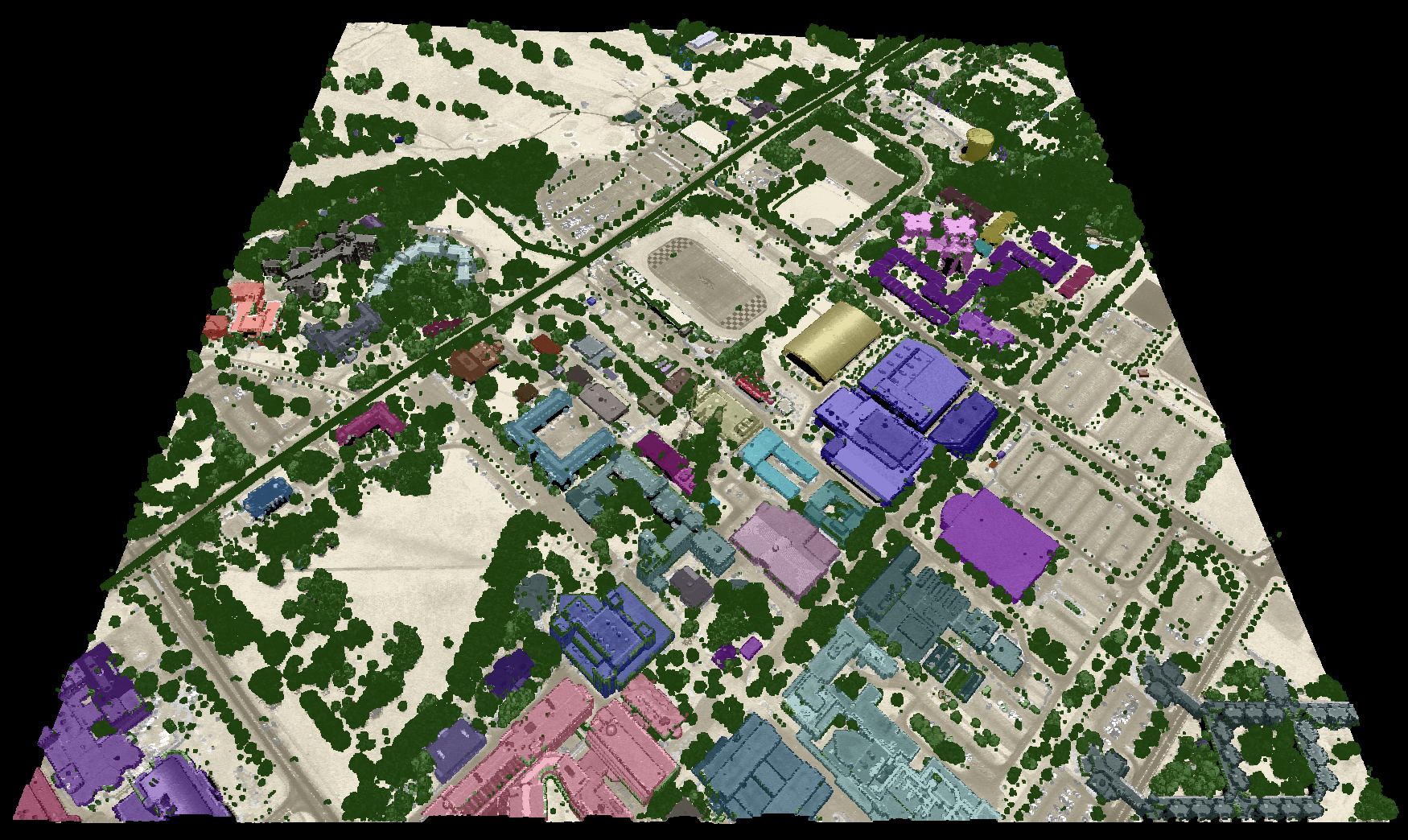
By default, the tool renders buildings in red (see table below). However, the tool also provides the option to
render each building in a unique colour (use_unique_clrs_for_buildings), providing a visually stunning
LiDAR-based map of built-up areas. When this option is selected, the user must also specify the radius
parameter, which determines the search distance used during the building segmentation operation. The radius
parameter is optional, and if unspecified (when the use_unique_clrs_for_buildings flag is used), a value of
2.0 will be used.
The specific colours used to render each point class can optionally be set by the user with the clr_str parameter.
The value of this parameter may list specific class values (0-18) and corresponding colour values in either a
red-green-blue (RGB) colour triplet form (i.e. (r, g, b)), or or a hex-colour, of either form #e6d6aa or
0xe6d6aa (note the # and 0x prefixes used to indicate hexadecimal numbers; also either lowercase or
capital letter values are acceptable). The following is an example of the a valid clr_str that sets the
ground (class 2) and high vegetation (class 5) colours used for rendering:
2: (184, 167, 108); 5: #9ab86c
Notice that 1) each class is separated by a semicolon (';'), 2) class values and colour values are separated by colons (':'), and 3) either RGB and hex-colour forms are valid.
If a clr_str parameter is not provided, the tool will use the default colours used for each class (see table below).
Class values are assumed to follow the class designations listed in the LAS specification:
| Classification Value | Meaning | Default Colour |
|---|---|---|
| 0 | Created never classified | |
| 1 | Unclassified | |
| 2 | Ground | |
| 3 | Low Vegetation | |
| 4 | Medium Vegetation | |
| 5 | High Vegetation | |
| 6 | Building | |
| 7 | Low Point (noise) | |
| 8 | Reserved | |
| 9 | Water | |
| 10 | Rail | |
| 11 | Road Surface | |
| 12 | Reserved | |
| 13 | Wire – Guard (Shield) | |
| 14 | Wire – Conductor (Phase) | |
| 15 | Transmission Tower | |
| 16 | Wire-structure Connector (e.g. Insulator) | |
| 17 | Bridge Deck | |
| 18 | High noise |
The point RGB colour values can be blended with the intensity data to create a particularly effective
visualization, further enhancing the visual interpretation of point return properties. The intensity_blending
parameter value, which must range from 0% (no intensity blending) to 100% (all intensity), is used to
set the degree of intensity/RGB blending.
Because the output file contains RGB colour data, it is possible that it will be larger than the input file. If the input file does contain valid RGB data, the output will be similarly sized, but the input colour data will be replaced in the output file with the point-return colours.
The output file can be visualized using any point cloud renderer capable of displaying point RGB information. We recommend the plas.io LiDAR renderer but many similar open-source options exist.
See Also
colourize_based_on_point_returns, lidar_colourize
Function Signature
def colourize_based_on_class(self, input_lidar: Optional[Lidar], intensity_blending_amount: float = 50.0, clr_str: str = "", use_unique_clrs_for_buildings: bool = False, search_radius: float = 2.0) -> Optional[Lidar]: ...
colourize_based_on_point_returns
License Information
Use of this function requires a license for Whitebox Workflows for Python Professional (WbW-Pro). Please visit www.whiteboxgeo.com to purchase a license.
Description
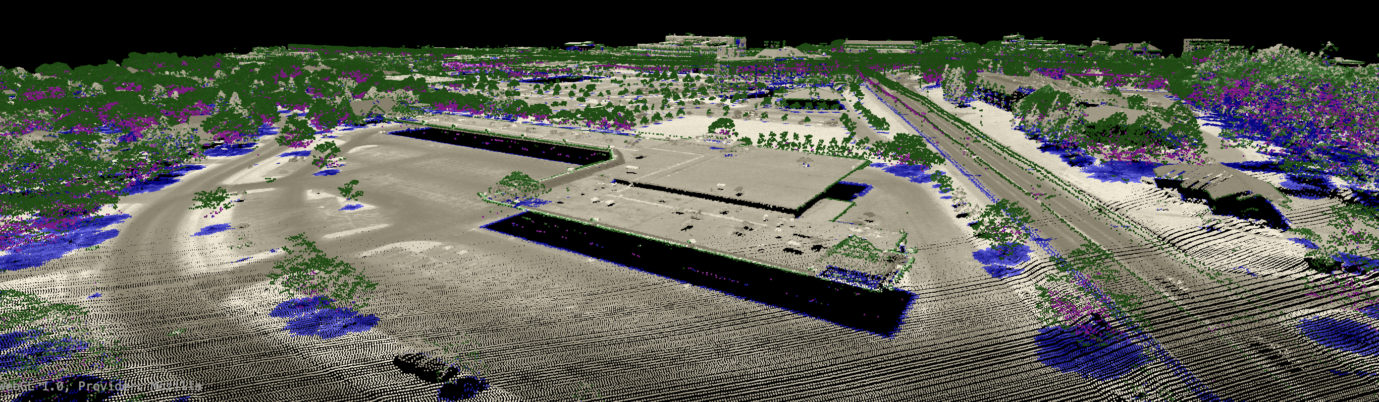
This tool sets the RGB colour values of a LiDAR point cloud (input) based on the point returns. It specifically
renders only-return, first-return, intermediate-return, and last-return points in different colours, storing
these data in the RGB colour data of the output LiDAR file (output). Colourizing the points in a LiDAR
point cloud based on return properties can aid with the visual inspection of point distributions, and therefore,
the quality assurance/quality control (QA/QC) of LiDAR data tiles. For example, this visualization process can
help to determine if there are areas of vegetation where there is insufficient coverage of ground points,
perhaps due to acquisition of the data during leaf-on conditions. There is often an assumption in LiDAR data
processing that the ground surface can be modelled using a subset of the only-return and last-return points
(beige and blue in the image below). However, under heavy forest cover, and in particular if the data were
collected during leaf-on conditions or if there is significant coverage of conifer trees, the only-return
and last-return points may be poor approximations of the ground surface. This tool can help to determine the
extent to which this is the case for a particular data set.
The specific colours used to render each return type can be set by the user with the only, first,
intermediate, and last parameters. Each parameter takes either a red-green-blue (RGB) colour triplet,
of the form (r,g,b), or a hex-colour, of either form #e6d6aa or 0xe6d6aa (note the # and 0x prefixes
used to indicate hexadecimal numbers; also either lowercase or capital letter values are acceptable).
The point RGB colour values can be blended with the intensity data to create a particularly effective
visualization, further enhancing the visual interpretation of point return properties. The intensity_blending
parameter value, which must range from 0% (no intensity blending) to 100% (all intensity), is used to
set the degree of intensity/RGB blending.
Because the output file contains RGB colour data, it is possible that it will be larger than the input file. If the input file does contain valid RGB data, the output will be similarly sized, but the input colour data will be replaced in the output file with the point-return colours.
The output file can be visualized using any point cloud renderer capable of displaying point RGB information. We recommend the plas.io LiDAR renderer but many similar open-source options exist.
This tool is a convenience function and can alternatively be achieved using the modify_lidar tool with the statement:
rgb=if(is_only, (230,214,170), if(is_last, (0,0,255), if(is_first, (0,255,0), (255,0,255))))
The colourize_based_on_point_returns tool is however significantly faster for this operation than the modify_lidar tool because the expression above must be executed dynamically for each point.
See Also
Function Signature
def colourize_based_on_point_returns(self, input_lidar: Optional[Lidar], intensity_blending_amount: float = 50.0, only_ret_colour: str = "(230,214,170)", first_ret_colour:str = "(0,140,0)", intermediate_ret_colour: str = "(255,0,255)", last_ret_colour: str = "(0,0,255)") -> Optional[Lidar]: ...
curvedness
License Information
Use of this function requires a license for Whitebox Workflows for Python Professional (WbW-Pro). Please visit www.whiteboxgeo.com to purchase a license.
Description
This tool calculates the curvedness (Koenderink and van Doorn, 1992) from a digital elevation model (DEM). Curvedness is the root mean square of maximal and minimal curvatures, and measures the magnitude of surface bending, regardless of shape (Florinsky, 2017). Curvedness is characteristically low-values for flat areas and higher for areas of sharp bending (Florinsky, 2017). The index is also inversely proportional with the size of the object (Koenderink and van Doorn, 1992). Curvedness has values equal to or greater than zero and is measured in units of m-1.
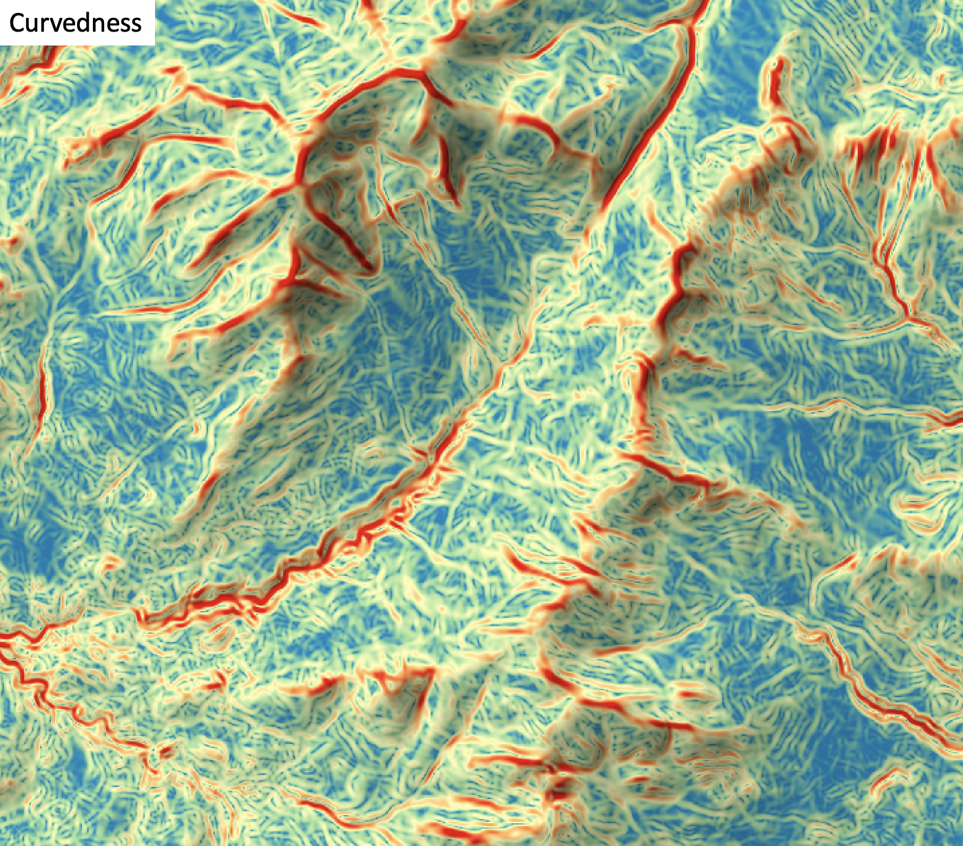
The user must specify the name of the input DEM (dem) and the output raster (output). The
The Z conversion factor (zfactor) is only important when the vertical and horizontal units are not the
same in the DEM. When this is the case, the algorithm will multiply each elevation in the DEM by the
Z Conversion Factor. Raw curvedness values are often challenging to visualize given their range and magnitude,
and as such the user may opt to log-transform the output raster (log). Transforming the values
applies the equation by Shary et al. (2002):
Θ' = sign(Θ) ln(1 + 10n|Θ|)
where Θ is the parameter value and n is dependent on the grid cell size.
For DEMs in projected coordinate systems, the tool uses the 3rd-order bivariate Taylor polynomial method described by Florinsky (2016). Based on a polynomial fit of the elevations within the 5x5 neighbourhood surrounding each cell, this method is considered more robust against outlier elevations (noise) than other methods. For DEMs in geographic coordinate systems (i.e. angular units), the tool uses the 3x3 polynomial fitting method for equal angle grids also described by Florinsky (2016).
References
Florinsky, I. (2016). Digital terrain analysis in soil science and geology. Academic Press.
Florinsky, I. V. (2017). An illustrated introduction to general geomorphometry. Progress in Physical Geography, 41(6), 723-752.
Koenderink, J. J., and Van Doorn, A. J. (1992). Surface shape and curvature scales. Image and vision computing, 10(8), 557-564.
Shary P. A., Sharaya L. S. and Mitusov A. V. (2002) Fundamental quantitative methods of land surface analysis. Geoderma 107: 1–32.
See Also
shape_index, minimal_curvature, maximal_curvature, tangential_curvature, profile_curvature, mean_curvature, gaussian_curvature
Function Signature
def curvedness(self, dem: Raster, log_transform: bool = False, z_factor: float = 1.0) -> Raster: ...
dbscan
License Information
Use of this function requires a license for Whitebox Workflows for Python Professional (WbW-Pro). Please visit www.whiteboxgeo.com to purchase a license.
Description
This tool performs an unsupervised DBSCAN clustering operation, based
on a series of input rasters (inputs). Each grid cell defines a stack of feature values (one value for
each input raster), which serves as a point within the multi-dimensional feature space. The DBSCAN
algorithm identifies clusters in feature space by identifying regions of high density (core points)
and the set of points connected to these high-density areas. Points in feature space that are not
connected to high-density regions are labeled by the DBSCAN algorithm as 'noise' and the associated
grid cell in the output raster (output) is assigned the nodata value. Areas of high density (i.e. core
points) are defined as those points for which the number of neighbouring points within a search distance
(search_dist) is greater than some user-defined minimum threshold (min_points).
The main advantages of the DBSCAN algorithm over other clustering methods, such as k-means (k_means_clustering), is that 1) you do not need to specify the number of clusters a priori, and 2) that the method does not make assumptions about the shape of the cluster (spherical in the k-means method). However, DBSCAN does assume that the density of every cluster in the data is approximately equal, which may not be a valid assumption. DBSCAN may also produce unsatisfactory results if there is significant overlap among clusters, as it will aggregate the clusters. Finding search distance and minimum core-point density thresholds that apply globally to the entire data set may be very challenging or impossible for certain applications.
The DBSCAN algorithm is based on the calculation of distances in multi-dimensional space. Feature scaling is
essential to the application of DBSCAN clustering, especially when the ranges of the features are different, for
example, if they are measured in different units. Without scaling, features with larger ranges will have
greater influence in computing the distances between points. The tool offers three options for feature-scaling (scaling),
including 'None', 'Normalize', and 'Standardize'. Normalization simply rescales each of the features onto
a 0-1 range. This is a good option for most applications, but it is highly sensitive to outliers because
it is determined by the range of the minimum and maximum values. Standardization
rescales predictors using their means and standard deviations, transforming the data into z-scores. This
is a better option than normalization when you know that the data contain outlier values; however, it does
does assume that the feature data are somewhat normally distributed, or are at least symmetrical in
distribution.
One should keep the impact of feature scaling in mind when setting the search_dist parameter. For
example, if applying normalization, the entire range of values for each dimension of feature space will
be bound within the 0-1 range, meaning that the search distance should be smaller than 1.0, and likely
significantly smaller. If standardization is used instead, features space is technically infinite,
although the vast majority of the data are likely to be contained within the range -2.5 to 2.5.
Because the DBSCAN algorithm calculates distances in feature-space, like many other related algorithms, it suffers from the curse of dimensionality. Distances become less meaningful in high-dimensional space because the vastness of these spaces means that distances between points are less significant (more similar). As such, if the predictor list includes insignificant or highly correlated variables, it is advisable to exclude these features during the model-building phase, or to use a dimension reduction technique such as principal_component_analysis to transform the features into a smaller set of uncorrelated predictors.
Memory Usage
The peak memory usage of this tool is approximately 8 bytes per grid cell × # predictors.
See Also
k_means_clustering, modified_k_means_clustering, principal_component_analysis
Function Signature
def dbscan(self, input_rasters: List[Raster], scaling_method: str = "none", search_distance: float = 1.0, min_points: int = 5) -> Raster: ...
dem_void_filling
License Information
Use of this function requires a license for Whitebox Workflows for Python Professional (WbW-Pro). Please visit www.whiteboxgeo.com to purchase a license.
Description
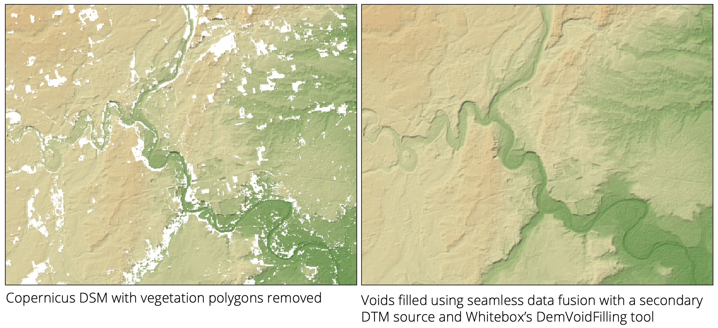
This tool implements a modified version of the Delta Surface Fill method of Grohman et al. (2006). It can
fill voids (i.e., data holes) contained within a digital elevation model (dem) by fusing the data with a
second DEM (fill) that defines the topographic surface within the void areas. The two surfaces are fused
seamlessly so that the transition from the source and fill surfaces is undetectable. The fill surface need
not have the same resolution as the source DEM.
The algorithm works by computing a DEM-of-difference (DoD) for each valid grid cell in the source DEM that also has a valid elevation in the corresponding location within the fill DEM. This difference surface is then used to define offsets within the near void-edge locations. The fill surface elevations are then combined with interpolated offsets, with the interpolation based on near-edge offsets, and used to define a new surface within the void areas of the source DEM in such a way that the data transitions seamlessly from the source data source to the fill data. The image below provides an example of this method.
The user must specify the mean_plane_dist parameter, which defines the distance (measured in grid cells)
within a void area from the void's edge. Grid cells within larger voids that are beyond this distance
from their edges have their vertical offsets, needed during the fusion of the DEMs, set to the mean offset
for all grid cells that have both valid source and fill elevations. Void cells that are nearer their void
edges have vertical offsets that are interpolated based on nearby offset values (i.e., the DEM of difference).
The interpolation uses inverse-distance weighted (IDW) scheme, with a user-specified weight parameter (weight_value).
The edge_treatment parameter describes how the data fusion operates at the edges of voids, i.e., the first line
of grid cells for which there are both source and fill elevation values. This parameter has values of "use DEM",
"use Fill", and "average". Grohman et al. (2006) state that sometimes, due to a weakened signal within these
marginal locations between the area of valid data and voids, the estimated elevation values are inaccurate. When
this is the case, it is best to use fill elevations in the transitional areas. If this isn't the case, the
"use DEM" is the better option. A compromise between the two options is to average the two elevation sources.
References
Grohman, G., Kroenung, G. and Strebeck, J., 2006. Filling SRTM voids: The delta surface fill method. Photogrammetric Engineering and Remote Sensing, 72(3), pp.213-216.
Function Signature
def dem_void_filling(self, dem: Raster, fill: Raster, mean_plane_dist: int = 20, edge_treatment: str = "dem", weight_value: float = 2.0) -> Raster: ...
depth_to_water
License Information
Use of this function requires a license for Whitebox Workflows for Python Professional (WbW-Pro). Please visit www.whiteboxgeo.com to purchase a license.
Description
This tool calculates the cartographic depth-to-water (DTW) index described by Murphy et al. (2009). The DTW index has been shown to be related to soil moisture, and is useful for identifying low-lying positions that are likely to experience surface saturated conditions. In this regard, it is similar to each of wetness_index, elevation_above_stream (HAND), and probability-of-depressions (i.e. stochastic_depression_analysis).

The index is the cumulative slope gradient along the least-slope path connecting each grid cell in an input DEM (dem) to
a surface water cell. Tangent slope (i.e. rise / run) is calculated for each grid cell based on the neighbouring elevation
values in the input DEM. The algorithm
operates much like a cost-accumulation analysis (cost_distance), where the cost of moving through a cell is determined
by the cell's tangent slope value and the distance travelled. Therefore, lower DTW values are associated with wetter soils and
higher values indicate drier conditions, over longer time periods. Areas of surface water have DTW values of zero. The user
must input surface water features, including vector stream lines (streams) and/or vector waterbody polygons
(lakes, i.e. lakes, ponds, wetlands, etc.). At least one of these two optional water feature inputs must be specified. The
tool internally rasterizes these vector features, setting the DTW value in the output raster to zero. DTW tends
to increase with greater distances from surface water features, and increases more slowly in flatter topography and more
rapidly in steeper settings. Murphy et al. (2009) state that DTW is a probablistic model that assumes uniform soil properties,
climate, and vegetation.
Note that DTW values are highly dependent upon the accuracy and extent of the input streams/lakes layer(s).
References
Murphy, PNC, Gilvie, JO, and Arp, PA (2009) Topographic modelling of soil moisture conditiTons: a comparison and verification of two models. European Journal of Soil Science, 60, 94–109, DOI: 10.1111/j.1365-2389.2008.01094.x.
See Also
wetness_index, elevation_above_stream, stochastic_depression_analysis
Function Signature
def depth_to_water(self, dem: Raster, streams: Optional[Vector] = None, lakes: Optional[Vector] = None) -> Raster: ...
difference_curvature
License Information
Use of this function requires a license for Whitebox Workflows for Python Professional (WbW-Pro). Please visit www.whiteboxgeo.com to purchase a license.
Description
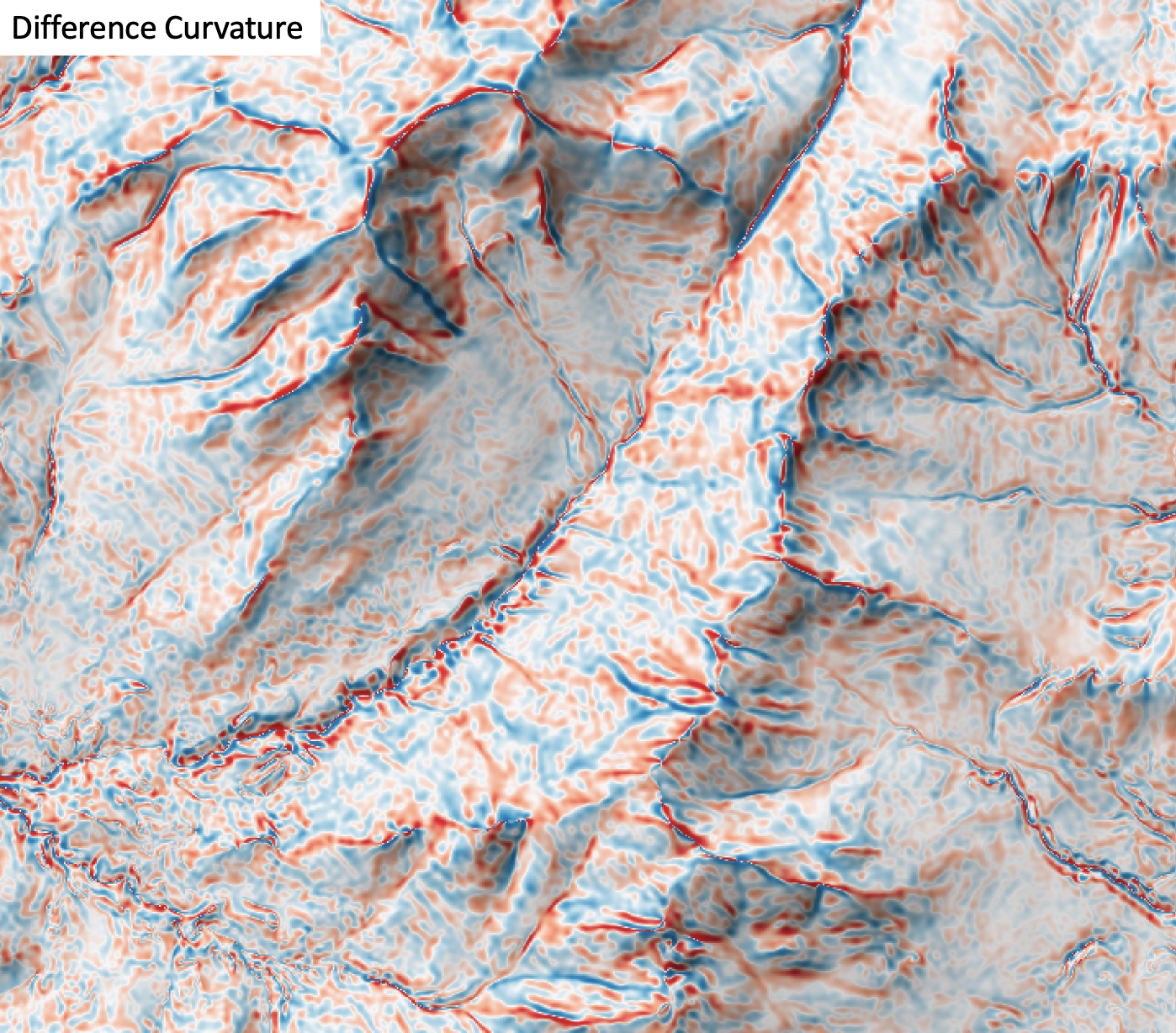
This tool calculates the difference curvature from a digital elevation model (DEM). Difference curvature is half of the difference between profile and tangential curvatures, sometimes called the vertical and horizontal curvatures (Shary, 1995). This variable has an unbounded range that can take either positive or negative values. Florinsky (2017) states that difference curvature measures the extent to which the relative deceleration of flows (measured by kv) is higher than flow convergence at a given point of the topographic surface. Difference curvature is measured in units of m-1.
The user must specify the name of the input DEM (dem) and the output raster (output). The
The Z conversion factor (zfactor) is only important when the vertical and horizontal units are not the
same in the DEM. When this is the case, the algorithm will multiply each elevation in the DEM by the
Z Conversion Factor. Curvature values are often very small and as such the user may opt to log-transform
the output raster (log). Transforming the values applies the equation by Shary et al. (2002):
Θ' = sign(Θ) ln(1 + 10n|Θ|)
where Θ is the parameter value and n is dependent on the grid cell size.
For DEMs in projected coordinate systems, the tool uses the 3rd-order bivariate Taylor polynomial method described by Florinsky (2016). Based on a polynomial fit of the elevations within the 5x5 neighbourhood surrounding each cell, this method is considered more robust against outlier elevations (noise) than other methods. For DEMs in geographic coordinate systems (i.e. angular units), the tool uses the 3x3 polynomial fitting method for equal angle grids also described by Florinsky (2016).
References
Florinsky, I. (2016). Digital terrain analysis in soil science and geology. Academic Press.
Florinsky, I. V. (2017). An illustrated introduction to general geomorphometry. Progress in Physical Geography, 41(6), 723-752.
Shary PA (1995) Land surface in gravity points classification by a complete system of curvatures. Mathematical Geology 27: 373–390.
Shary P. A., Sharaya L. S. and Mitusov A. V. (2002) Fundamental quantitative methods of land surface analysis. Geoderma 107: 1–32.
See Also
profile_curvature, tangential_curvature, rotor, minimal_curvature, maximal_curvature, mean_curvature, gaussian_curvature
Function Signature
def difference_curvature(self, dem: Raster, log_transform: bool = False, z_factor: float = 1.0) -> Raster: ...
evaluate_training_sites
License Information
Use of this function requires a license for Whitebox Workflows for Python Professional (WbW-Pro). Please visit www.whiteboxgeo.com to purchase a license.
Description
This tool performs an evaluation of the reflectance properties of multi-spectral image dataset for a
group of digitized class polygons. This is often viewed as the first step in a supervised classification
procedure, such as those performed using the min_dist_classification or parallelepiped_classification
tools. The analysis is based on a series of one or more input images (inputs) and an input polygon
vector file (polys). The user must also specify the attribute name (field), within the attribute
table, containing the class ID associated with each feature in input the polygon vector. A single class
may be designated by multiple polygon features in the test site polygon vector. Note that the
input polygon file is generally created by digitizing training areas of exemplar reflectance properties for each
class type. The input polygon vector should be in the same coordinate system as the input multi-spectral images.
The input images must represent a multi-spectral data set made up of individual bands.
Do not input colour composite images. Lastly, the user must specify the name of the output HTML file.
This file will contain a series of box-and-whisker plots, one
for each band in the multi-spectral data set, that visualize the distribution of each class in the
associated bands. This can be helpful in determining the overlap between spectral properties for the
classes, which may be useful if further class or test site refinement is necessary. For a subsequent
supervised classification to be successful, each class should not overlap significantly with the other
classes in at least one of the input bands. If this is not the case, the user may need to refine
the class system.

See Also
min_dist_classification, parallelepiped_classification
Function Signature
def evaluate_training_sites(self, input_rasters: List[Raster], training_polygons: Vector, class_field_name: str, output_html_file: str) -> None: ...
filter_lidar
License Information
Use of this function requires a license for Whitebox Workflows for Python Professional (WbW-Pro). Please visit www.whiteboxgeo.com to purchase a license.
Description
The FilterLidar tool is a very powerful tool for filtering points within a LiDAR point cloud based on point
properties. Complex filter statements (statement) can be used to include or exclude points in the
output file (output).
Note that if the user does not specify the optional input LiDAR file (input), the tool will search for all
valid LiDAR (*.las, *.laz, *.zlidar) files contained within the current working directory. This feature can be useful
for processing a large number of LiDAR files in batch mode. When this batch mode is applied, the output file
names will be the same as the input file names but with a '_filtered' suffix added to the end.
Points are either included or excluded from the output file by creating conditional filter statements. Statements must be valid Rust syntax and evaluate to a Boolean. Any of the following variables are acceptable within the filter statement:
| Variable Name | Description |
|---|---|
| x | The point x coordinate |
| y | The point y coordinate |
| z | The point z coordinate |
| intensity | The point intensity value |
| ret | The point return number |
| nret | The point number of returns |
| is_only | True if the point is an only return (i.e. ret == nret == 1), otherwise false |
| is_multiple | True if the point is a multiple return (i.e. nret > 1), otherwise false |
| is_early | True if the point is an early return (i.e. ret == 1), otherwise false |
| is_intermediate | True if the point is an intermediate return (i.e. ret > 1 && ret < nret), otherwise false |
| is_late | True if the point is a late return (i.e. ret == nret), otherwise false |
| is_first | True if the point is a first return (i.e. ret == 1 && nret > 1), otherwise false |
| is_last | True if the point is a last return (i.e. ret == nret && nret > 1), otherwise false |
| class | The class value in numeric form, e.g. 0 = Never classified, 1 = Unclassified, 2 = Ground, etc. |
| is_noise | True if the point is classified noise (i.e. class == 7 |
| is_synthetic | True if the point is synthetic, otherwise false |
| is_keypoint | True if the point is a keypoint, otherwise false |
| is_withheld | True if the point is withheld, otherwise false |
| is_overlap | True if the point is an overlap point, otherwise false |
| scan_angle | The point scan angle |
| scan_direction | True if the scanner is moving from the left towards the right, otherwise false |
| is_flightline_edge | True if the point is situated along the filightline edge, otherwise false |
| user_data | The point user data |
| point_source_id | The point source ID |
| scanner_channel | The point scanner channel |
| time | The point GPS time, if it exists, otherwise 0 |
| red | The point red value, if it exists, otherwise 0 |
| green | The point green value, if it exists, otherwise 0 |
| blue | The point blue value, if it exists, otherwise 0 |
| nir | The point near infrared value, if it exists, otherwise 0 |
| pt_num | The point number within the input file |
| n_pts | The number of points within the file |
| min_x | The file minimum x value |
| mid_x | The file mid-point x value |
| max_x | The file maximum x value |
| min_y | The file minimum y value |
| mid_y | The file mid-point y value |
| max_y | The file maximum y value |
| min_z | The file minimum z value |
| mid_z | The file mid-point z value |
| max_z | The file maximum z value |
| dist_to_pt | The distance from the point to a specified xy or xyz point, e.g. dist_to_pt(562500, 4819500) or dist_to_pt(562500, 4819500, 320) |
| dist_to_line | The distance from the point to the line passing through two xy points, e.g. dist_to_line(562600, 4819500, 562750, 4819750) |
| dist_to_line_seg | The distance from the point to the line segment defined by two xy end-points, e.g. dist_to_line_seg(562600, 4819500, 562750, 4819750) |
| within_rect | 1 if the point falls within the bounds of a 2D or 3D rectangle, otherwise 0. Bounds are defined as within_rect(ULX, ULY, LRX, LRY) or within_rect(ULX, ULY, ULZ, LRX, LRY, LRZ) |
In addition to the point properties defined above, if the user applies the lidar_eigenvalue_features
tool on the input LiDAR file, the filter_lidar tool will automatically read in the additional *.eigen
file, which include the eigenvalue-based point neighbourhood measures, such as lambda1, lambda2, lambda3,
linearity, planarity, sphericity, omnivariance, eigentropy, slope, and residual. See the
lidar_eigenvalue_features documentation for details on each of these metrics describing the structure
and distribution of points within the neighbourhood surrounding each point in the LiDAR file.
Statements can be as simple or complex as desired. For example, to filter out all points that are classified noise (i.e. class numbers 7 or 18):
!is_noise
The following is a statement to retain only the late returns from the input file (i.e. both last and single returns):
ret == nret
Notice that equality uses the == symbol an inequality uses the != symbol. As an equivalent to the above
statement, we could have used the is_late point property:
is_late
If we want to remove all points outside of a range of xy values:
x >= 562000 && x <= 562500 && y >= 4819000 && y <= 4819500
Notice how we can combine multiple constraints using the && (logical AND) and || (logical OR) operators.
As an alternative to the above statement, we could have used the within_rect function:
within_rect(562000, 4819500, 562500, 4819000)
If we want instead to exclude all of the points within this defined region, rather than to retain them, we
simply use the ! (logial NOT):
!(x >= 562000 && x <= 562500 && y >= 4819000 && y <= 4819500)
or, simply:
!within_rect(562000, 4819500, 562500, 4819000)
If we need to find all of the ground points within 150 m of (562000, 4819500), we could use:
class == 2 && dist_to_pt(562000, 4819500) <= 150.0
The following statement outputs all non-vegetation classed points in the upper-right quadrant:
!(class == 3 && class != 4 && class != 5) && x < min_x + (max_x - min_x) / 2.0 && y > max_y - (max_y - min_y) / 2.0
As demonstrated above, the filter_lidar tool provides an extremely flexible, powerful, and easy means for retaining and removing points from point clouds based on any of the common LiDAR point attributes.
See Also
filter_lidar_classes, filter_lidar_scan_angles, modify_lidar, erase_polygon_from_lidar, clip_lidar_to_polygon, sort_lidar, lidar_eigenvalue_features
Function Signature
def filter_lidar(self, statement: str, input_lidar: Optional[Lidar]) -> Optional[Lidar]: ...
filter_lidar_by_percentile
License Information
Use of this function requires a license for Whitebox Workflows for Python Professional (WbW-Pro). Please visit www.whiteboxgeo.com to purchase a license.
Description
This tool can be used to extract a subset of points from an input LiDAR point cloud (input_lidar) that correspond
to a user-specified percentile of the points within the local neighbourhood. The algorithm works by overlaying a
grid of a specified size (block_size). The group of LiDAR points contained within each block in the superimposed
grid are identified and are sorted by elevation. The point with the elevation that corresponds most closely to the
specified percentile is then inserted into the output LiDAR point cloud. For example, if percentile = 0.0, the
lowest point within each block will be output, if percentile = 100.0 the highest point will be output, and if
percentile = 50.0 the point that is nearest the median elevation will be output. Notice that the lower the number
of points contained within a block, the more approximate the calculation will be. For example, if a block only contains
three points, no single point occupies the 25th percentile. The equation that is used to identify the closest
corresponding point (zero-based) from a list of n sorted by elevation values is:
point_num = ⌊percentile / 100.0 * (n - 1)⌉
Increasing the block size (default is 1.0 xy-units) will increase the average number of points within blocks, allowing for a more accurate percentile calculation.
Like many of the LiDAR functions, the input LiDAR point cloud (input_lidar) is optional. If an input LiDAR file
is not specified, the tool will search for all valid LiDAR (*.las, *.laz, *.zlidar) files contained within the current
working directory. This feature can be very useful when you need to process a large number of LiDAR files contained
within a directory. This batch processing mode enables the function to run in a more optimized parallel manner.
When run in this batch mode, no output LiDAR object will be created. Instead the function will create
an output file (saved to disc) with the same name as each input LiDAR file, but with the .tif extension. This can provide a very
efficient means for processing extremely large LiDAR data sets.
See Also
filter_lidar, lidar_block_minimum, lidar_block_maximum
Function Signature
def filter_lidar_by_percentile(self, input_lidar: Optional[Lidar], percentile: float = 0.0, block_size: float = 1.0) -> Optional[Lidar]: ...
filter_lidar_by_reference_surface
License Information
Use of this function requires a license for Whitebox Workflows for Python Professional (WbW-Pro). Please visit www.whiteboxgeo.com to purchase a license.
Description
This tool can be used to extract a subset of points from an input LiDAR point cloud (input_lidar) that satisfy a
query relation with a user-specified raster reference surface (ref_surface). For example, you may use this
function to extract all of the points that are below (query="<" or query="<=") or above (query=">" or query=">=")
a surface model. The default query mode is "within" (i.e. query="within"), which extracts all of the points that
are within a specified absolute vertical distance (threshold) of the surface. Notice that the threshold parameter
is ignored for query types other than "within".
By default, the function will return a point cloud containing only the subset of points in the input dataset that satisfy
the condition of the query. Setting the classify parameter to True modifies this behaviour such that the output
point cloud will contain all of the points within the input dataset, but will have the classification value of the
query-satifying points will be set to the true_class_value parameter (0-255) and points that do not satisfy the query
will be assigned the false_class_value (0-255). By setting the preserve_classes paramter to True, all points that do not
satisfy the query will have unmodified class values from the input dataset.
Unlike many of the LiDAR functions, this function does not have a batch mode and operates on single tiles only.
See Also
Function Signature
def filter_lidar_by_reference_surface(self, input_lidar: Lidar, ref_surface: Raster, query: str = "within", threshold: float = 0.0) -> Lidar: ...
fix_dangling_arcs
License Information
Use of this function requires a license for Whitebox Workflows for Python Professional (WbW-Pro). Please visit www.whiteboxgeo.com to purchase a license.
Description
This tool can be used to fix undershot and overshot arcs, two common topological errors,
in an input vector lines file (input). In addition to the input lines vector, the user must
also specify the output vector (output) and the snap distance (snap). All dangling arcs
that are within this threshold snap distance of another line feature will be connected to the
neighbouring feature. If the input lines network is a vector stream network, users are advised
to apply the repair_stream_vector_topology tool instead.

See Also
repair_stream_vector_topology, clean_vector
Function Signature
def fix_dangling_arcs(self, input: Vector, snap_dist: float) -> Vector: ...
fuzzy_knn_classification
License Information
Use of this function requires a license for Whitebox Workflows for Python Professional (WbW-Pro). Please visit www.whiteboxgeo.com to purchase a license.
Description
This tool performs a supervised fuzzy k-nearest neighbour (k-NN) classification
using multiple predictor rasters (inputs), or features, and training data (training). This implementation is based
on the Keller et al. (1985) algorithm. The function can be used to model the spatial distribution of class data,
such as land-cover type, soil class, or vegetation type. The training data take the form of an input vector Shapefile
containing a set of points or polygons, for which the known class information is contained within a field (field) of
the attribute table. Each grid cell defines a stack of feature values (one value for each input raster), which serves as
a point within the multi-dimensional feature space. The algorithm works by identifying a user-defined number (k, -k) of
feature-space neighbours from the training set for each grid cell. The class that is then assigned to
the grid cell in the output raster (output) is then determined as a distance-weighted sum of classes among the
set of training data neighbours. The implementation uses Keller et al.'s (1985) third method of assigning membership to
training points. This method attempts to "fuzzify" the memberships of the labeled samples, which are in the class regions
intersecting in the sample space, and leaves the samples that are well away from this area with complete membership in the
known class. As a result, an unknown sample lying in this intersecting region will be influenced to a lesser extent by the
labeled samples of the training data that are in the "fuzzy" area of the class boundary.
Fuzzy kNN has often been found to outperform the regular kNN method for classification problems and has the extra advantage of outputing information about class membership uncertainty. This function optionally outputs two rasters, the first being the classified image (i.e., the crisply classified image determined by assigning each cell to the class for which the membership probability is highest) and the second raster indicating the membership probability. Grid cells with relatively low membership probability are indicative of greater uncertainty associated with the classification. Note that because membership probabilities across all classes must sum to 1.0 for each grid cell, the lowest possible membership probability for the "winning" class is 1 / N, where N is the number of input features. Examining the membership probability raster can provide insight into how the information class structure or training data sets can be improved, if for example, certain classes are commonly associated with lower membership probability.
The function uses leave-one-out-cross-validation (LOOCV) to measure the accuracy of the fit model. This approach is used to calculate the overall accuracy and Cohen's kappa index of agreement.
Note that the output image parameter (output) is optional. When unspecified, the tool will simply
report the model accuracy statistics and variable importance, allowing the user to experiment with different parameter
settings and input predictor raster combinations to optimize the model before applying it to classify
the whole image data set.
Like all supervised classification methods, this technique relies heavily on proper selection of training data. Training sites are exemplar areas/points of known and representative class value (e.g. land cover type). The algorithm determines the feature signatures of the pixels within each training area. In selecting training sites, care should be taken to ensure that they cover the full range of variability within each class. Otherwise the classification accuracy will be impacted. If possible, multiple training sites should be selected for each class. It is also advisable to avoid areas near the edges of class objects (e.g. land-cover patches), where mixed pixels may impact the purity of training site values.
After selecting training sites, the feature value distributions of each class type can be assessed using the evaluate_training_sites tool. In particular, the distribution of class values should ideally be non-overlapping in at least one feature dimension.
The fuzzy k-NN algorithm is based on the calculation of distances in multi-dimensional space. Feature scaling is
essential to the application of fuzzy k-NN modelling, especially when the ranges of the features are different, for
example, if they are measured in different units. Without scaling, features with larger ranges will have
greater influence in computing the distances between points. The tool offers three options for feature-scaling (scaling),
including 'None', 'Normalize', and 'Standardize'. Normalization simply rescales each of the features onto
a 0-1 range. This is a good option for most applications, but it is highly sensitive to outliers because
it is determined by the range of the minimum and maximum values. Standardization
rescales predictors using their means and standard deviations, transforming the data into z-scores. This
is a better option than normalization when you know that the data contain outlier values; however, it does
does assume that the feature data are somewhat normally distributed, or are at least symmetrical in
distribution.
Because the fuzzy k-NN algorithm calculates distances in feature-space, like many other related algorithms, it suffers from the curse of dimensionality. Distances become less meaningful in high-dimensional space because the vastness of these spaces means that distances between points are less significant (more similar). As such, if the predictor list includes insignificant or highly correlated variables, it is advisable to exclude these features during the model-building phase, or to use a dimension reduction technique such as principal_component_analysis to transform the features into a smaller set of uncorrelated predictors.
Note that the knn_regression tool can be used to apply the k-NN method to the modelling of continuous data.
Memory Usage
The peak memory usage of this tool is approximately 8 bytes per grid cell × # predictors.
References
Keller, J. M., Gray, M. R., and Givens, J. A. (1985). A fuzzy k-nearest neighbor algorithm. IEEE transactions on systems, man, and cybernetics, (4), 580-585.
See Also
knn_classification,, knn_regression, random_forest_classification, svm_classification, parallelepiped_classification, evaluate_training_sites
Function Signature
def knn_classification(self, input_rasters: List[Raster], training_data: Vector, class_field_name: str, scaling_method: str = "none", k: int = 5, test_proportion: float = 0.2, use_clipping: bool = False, create_output: bool = False) -> Optional[Raster]: ...
generalize_classified_raster
License Information
Use of this function requires a license for Whitebox Workflows for Python Professional (WbW-Pro). Please visit www.whiteboxgeo.com to purchase a license.
Description
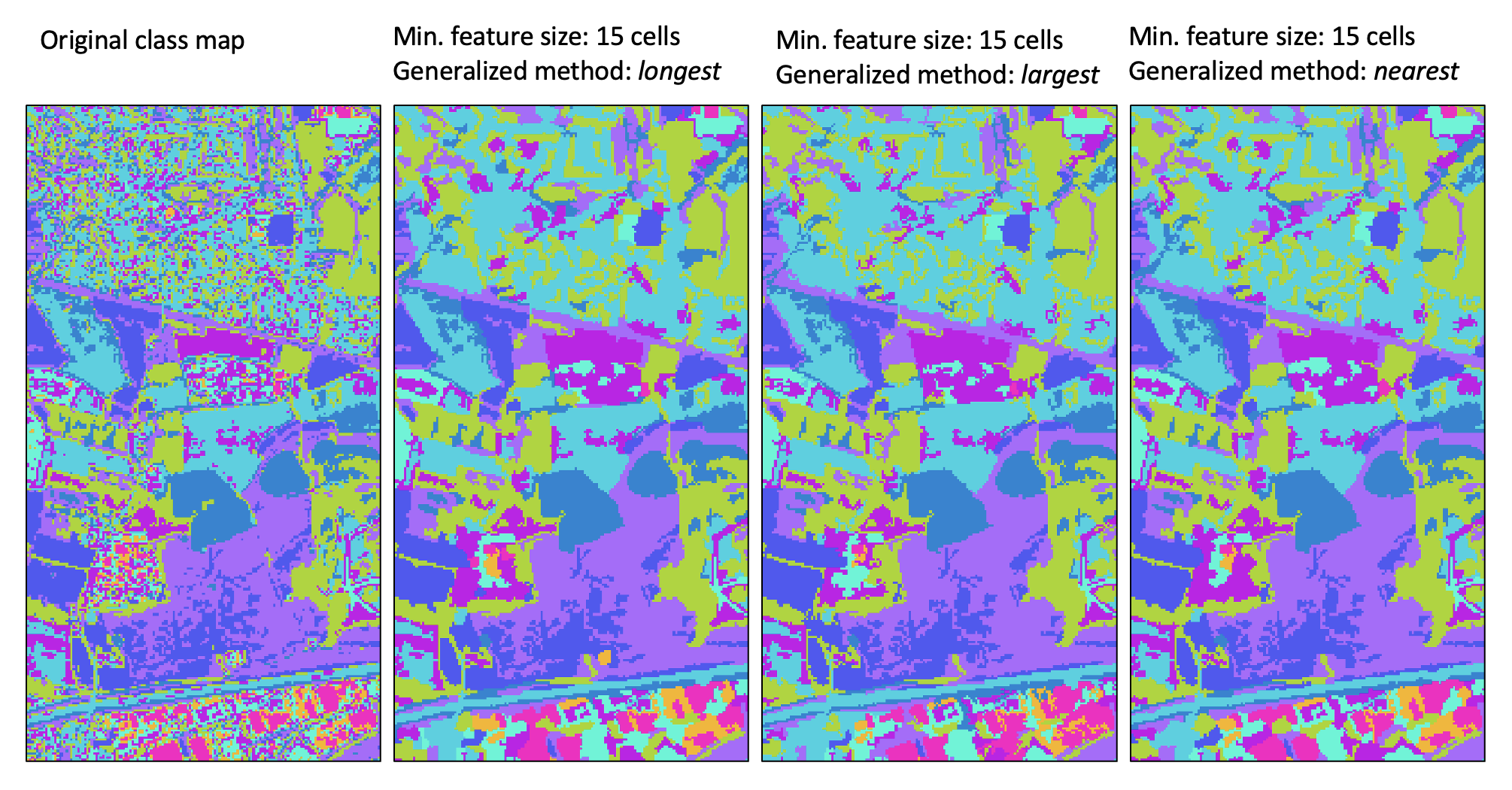
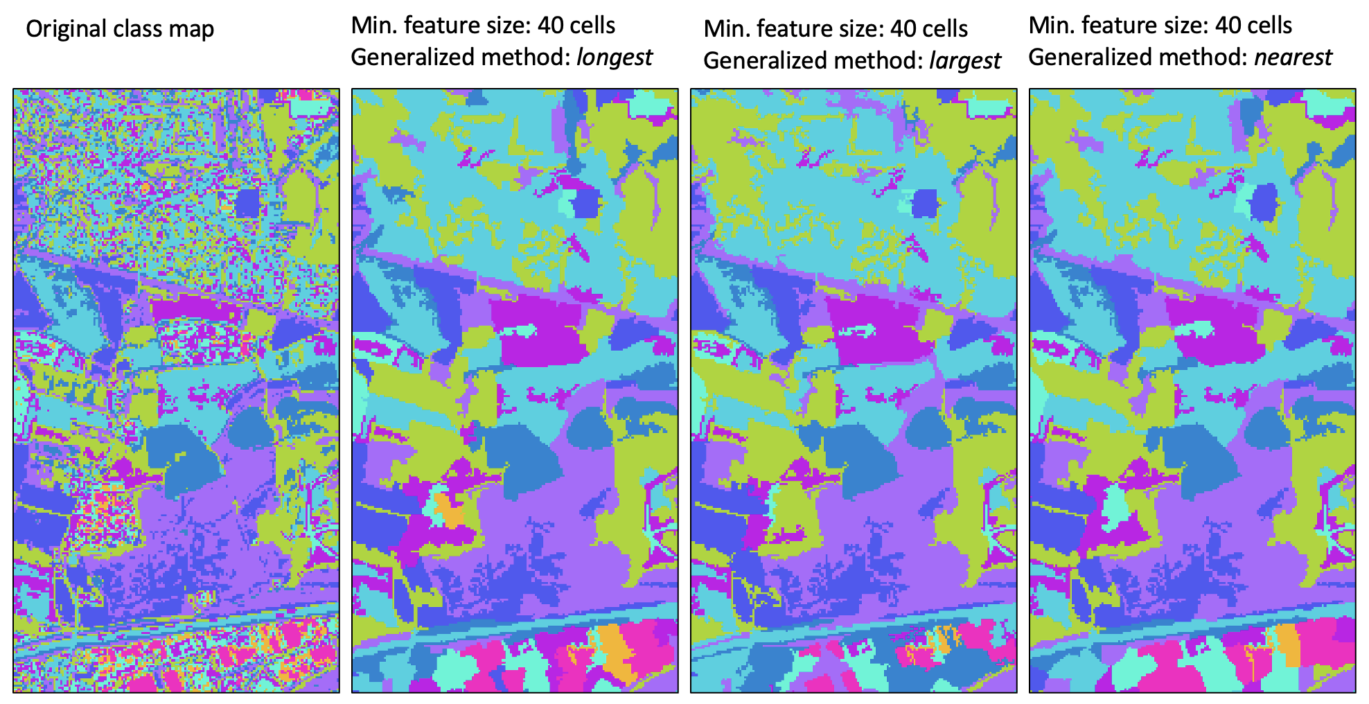
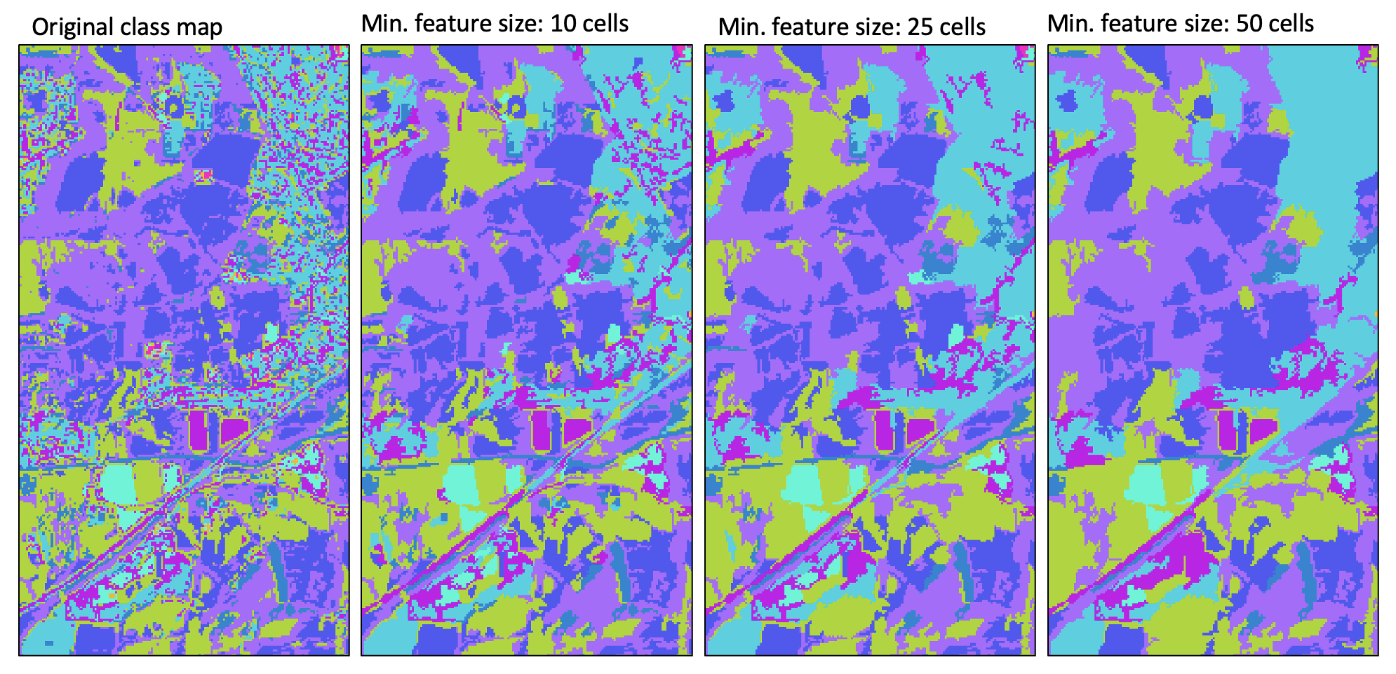
This tool can be used to generalize a raster containing class or object features. Such rasters are usually derived from some classification procedure (e.g. image classification and landform classification), or as the output of a segmentation procedure (image_segmentation). Rasters that are created in this way often contain many very small features that make their interpretation, or vectorization, challenging. Therefore, it is common for practitioners to remove the smaller features. Many different approaches have been used for this task in the past. For example, it is common to remove small features using a filtering based approach (majority_filter). While this can be an effective strategy, it does have the disadvantage of modifying all of the boundaries in the class raster, including those that define larger features. In many applications, this can be a serious issue of concern.
The generalize_classified_raster tool offers an alternative method for simplifying class rasters.
The process begins by identifying each contiguous group of cells in the input (i.e. a clumping
operation) and then defines the subset of features that are smaller than the user-specified minimum
feature size (min_size), in grid cells. This set of small features is then dealt with using
one of three methods (method). In the first method (longest), a small feature may be reassigned the class value
of the neighbouring feature with the longest shared border. The sum of the neighbouring
feature size and the small feature size must be larger than the specified size threshold, and the tool will iterate through this
process of reassigning feature values to neighbouring values until each small feature has been resolved.
The second method, largest, operates in much the same way as the first, except that objects are reassigned the value of the largest neighbour. Again, this process of reassigning small feature values iterates until every small feature has been reassigned to a large neighbouring feature.
The third and last method (nearest) takes a different approach to resolving the reassignment of small features. Using the nearest generalization approach, each grid cell contained within a small feature is reassigned the value of the nearest large neighbouring feature. When there are two or more neighbouring features that are equally distanced to a small feature cell, the cell will be reassigned to the largest neighbour. Perhaps the most significant disadvantage of this approach is that it creates a new artificial boundary in the output image that is not contained within the input class raster. That is, with the previous two methods, boundaries associated with smaller features in the input images are 'erased' in the output map, but every boundary in the output raster exactly matches boundaries within the input raster (i.e. the output boundaries are a subset of the input feature boundaries). However, with the nearest method, artificial boundaries, determined by the divide between nearest neighbours, are introduced to the output raster and these new feature boundaries do not have any basis in the original classification/segmentation process. Thus caution should be exercised when using this approach, especially when larger minimum size thresholds are used. The longest method is the recommended approach to class feature generalization.
For a video tutorial on how to use the generalize_classified_raster tool, see this YouTube video.
See Also
generalize_with_similarity, majority_filter, image_segmentation
Function Signature
def generalize_classified_raster(self, raster: Raster, area_threshold: int = 5, method: str = "longest") -> Raster: ...
generalize_with_similarity
License Information
Use of this function requires a license for Whitebox Workflows for Python Professional (WbW-Pro). Please visit www.whiteboxgeo.com to purchase a license.
Description
This tool can be used to generalize a raster containing class features (input) by reassigning
the identifier values of small features (min_size) to those of neighbouring features. Therefore, this tool
performs a very similar operation to the generalize_classified_raster tool. However, while the
generalize_classified_raster tool re-labels small features based on the geometric properties of
neighbouring features (e.g. neighbour with the longest shared border, largest neighbour, or
nearest neighbour), the generalize_with_similarity tool reassigns feature labels based on
similarity with neighbouring features. Similarity is determined using a series of input similarity
criteria rasters (similarity), which may be factors used in the creation of the input
class raster. For example, the similarlity rasters may be bands of multi-spectral imagery, if the
input raster is a classified land-cover map, or DEM-derived land surface parameters, if the input
raster is a landform class map.
The tool works by identifying each contiguous group of pixels (features) in the input class raster (input),
i.e. a clumping operation. The mean value is then calculated for each feature and each similarity
input, which defines a multi-dimensional 'similarity centre point' associated with each feature. It should be noted
that the similarity raster data are standardized prior to calculating these centre point values.
Lastly, the tool then reassigns the input label values of all features smaller than the user-specified
minimum feature size (min_size) to that of the neighbouring feature with the shortest distance
between similarity centre points.
For small features that are entirely enclosed by a single larger feature, this process will result in the same generalization solution presented by any of the geometric-based methods of the generalize_classified_raster tool. However, for small features that have more than one neighbour, this tool may provide a superior generalization solution than those based solely on geometric information.
For a video tutorial on how to use the generalize_with_similarity tool, see this YouTube video.
See Also
generalize_classified_raster, majority_filter, image_segmentation
Function Signature
def generalize_with_similarity(self, raster: Raster, similarity_rasters: List[Raster], area_threshold: int = 5) -> Raster: ...
generating_function
License Information
Use of this function requires a license for Whitebox Workflows for Python Professional (WbW-Pro). Please visit www.whiteboxgeo.com to purchase a license.
Description
This tool calculates the generating function (Shary and Stepanov, 1991) from a digital elevation model (DEM). Florinsky (2016) describes generating function as a measure for the deflection of tangential curvature from loci of extreme curvature of the topographic surface. Florinsky (2016) demonstrated the application of this variable for identifying landscape structural lines, i.e. ridges and thalwegs, for which the generating function takes values near zero. Ridges coincide with divergent areas where generating function is approximately zero, while thalwegs are associated with convergent areas with generating function values near zero. This variable has positive values, zero or greater and is measured in units of m-2.
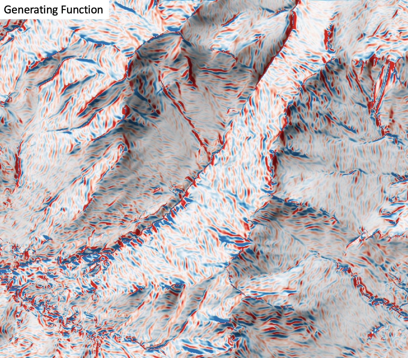
The user must specify the name of the input DEM (dem) and the output raster (output). The
The Z conversion factor (zfactor) is only important when the vertical and horizontal units are not the
same in the DEM. When this is the case, the algorithm will multiply each elevation in the DEM by the
Z Conversion Factor. Raw generating function values are often challenging to visualize given their range and magnitude,
and as such the user may opt to log-transform the output raster (log). Transforming the values
applies the equation by Shary et al. (2002):
Θ' = sign(Θ) ln(1 + 10n|Θ|)
where Θ is the parameter value and n is dependent on the grid cell size.
This tool uses the 3rd-order bivariate Taylor polynomial method described by Florinsky (2016). Based on a polynomial fit of the elevations within the 5x5 neighbourhood surrounding each cell, this method is considered more robust against outlier elevations (noise) than other methods. For DEMs in geographic coordinate systems, however, this tool cannot use the same 3x3 polynomial fitting method for equal angle grids, also described by Florinsky (2016), that is used by the other curvature tools in this software. That is because generating function uses 3rd order partial derivatives, which cannot be calculated using the 9 elevations in a 3x3; more elevation values are required (i.e. a 5x5 window). Thus, this tool uses the same 5x5 method used for DEMs in projected coordinate systems, and calculates the average linear distance between neighbouring cells in the vertical and horizontal directions using the Vincenty distance function. Note that this may cause a notable slow-down in algorithm performance and has a lower accuracy than would be achieved using an equal angle method, because it assumes a square pixel (in linear units).
References
Florinsky, I. (2016). Digital terrain analysis in soil science and geology. Academic Press.
Florinsky, I. V. (2017). An illustrated introduction to general geomorphometry. Progress in Physical Geography, 41(6), 723-752.
Koenderink, J. J., and Van Doorn, A. J. (1992). Surface shape and curvature scales. Image and vision computing, 10(8), 557-564.
Shary P. A., Sharaya L. S. and Mitusov A. V. (2002) Fundamental quantitative methods of land surface analysis. Geoderma 107: 1–32.
Shary P. A. and Stepanov I. N. (1991) Application of the method of second derivatives in geology. Transactions (Doklady) of the USSR Academy of Sciences, Earth Science Sections 320: 87–92.
See Also
shape_index, minimal_curvature, maximal_curvature, tangential_curvature, profile_curvature, mean_curvature, gaussian_curvature
Function Signature
def generating_function(self, dem: Raster, log_transform: bool = False, z_factor: float = 1.0) -> Raster: ...
horizon_area
License Information
Use of this function requires a license for Whitebox Workflows for Python Professional (WbW-Pro). Please visit www.whiteboxgeo.com to purchase a license.
This tool calculates horizon area, i.e., the area of the horizon polygon centered on each point in an
input digital elevation model (DEM). Horizon area is therefore conceptually related to the
viewhed and visibility_index
functions. Horizon area can be thought of as an approximation of the viewshed area and is therefore
faster to calculate a spatial distribution of compared with the visibility index. Horizon area is
measured in hectares.
The user must specify an input DEM (dem), the azimuth fraction (az_fraction), the maximum search
distance (max_dist), and the height offset of the observer (observer_hgt_offset). The input DEM
should usually be a digital surface model (DSM) that contains significant off-terrain objects. Such a
model, for example, could be created using the first-return points of a LiDAR data set, or using the
lidar_digital_surface_model tool. The azimuth
fraction should be an even divisor of 360-degrees and must be between 1-45 degrees.
The tool operates by calculating horizon angle (see horizon_angle)
rasters from the DSM based on the user-specified azimuth fraction (az_fraction). For example, if an azimuth
fraction of 15-degrees is specified, horizon angle rasters would be calculated for the solar azimuths 0,
15, 30, 45... A horizon angle raster evaluates the vertical angle between each grid cell in a DSM and a
distant obstacle (e.g. a mountain ridge, building, tree, etc.) that obscures the view in a specified
direction. In calculating horizon angle, the user must specify the maximum search distance (max_dist),
in map units, beyond which the query for higher, more distant objects will cease. This parameter strongly
impacts the performance of the function, with larger values resulting in significantly longer processing-times.
With each evaluated direction, the coordinates of the horizon point is determined, using the azimuth and the distance to horizon, with each point then serving as a vertex in a horizon polygon. The shoelace algorithm is used to measure the area of each horizon polgon for the set of grid cells, which is then reported in the output raster.
The observer_hgt_offset parameter can be used to add an increment to the source cell's elevation. For
example, the following image shows the spatial pattern derived from a LiDAR DSM using observer_hgt_offset = 0.0:
Notice that there are several places, plarticularly on the flatter rooftops, where the local noise in the LiDAR DEM, associated with the individual scan lines, has resulted in a noisy pattern in the output. By adding a small height offset of the scale of this noise variation (0.15 m), we see that most of this noisy pattern is removed in the output below:
As another example, in the image below, the observer_hgt_offset parameter has been used to measure
the pattern of the index at a typical human height (1.7 m):
Notice how at this height a much larger area becomes visible on some of the flat rooftops where a guard wall prevents further viewing areas at shorter observer heights.
See Also
sky_view_factor, average_horizon_distance, openness, lidar_digital_surface_model, horizon_angle
Function Signature
def horizon_area(self, dem: Raster, az_fraction: float = 5.0, max_dist: float = float('inf'), observer_hgt_offset: float = 0.0) -> Raster: ...
horizontal_excess_curvature
License Information
Use of this function requires a license for Whitebox Workflows for Python Professional (WbW-Pro). Please visit www.whiteboxgeo.com to purchase a license.
Description
This tool calculates the horizontal excess curvature from a digital elevation model (DEM). Horizontal excess curvature is the difference of tangential (horizontal) and minimal curvatures at a location (Shary, 1995). This variable has positive values, zero or greater. Florinsky (2017) states that horizontal excess curvature measures the extent to which the bending of a normal section tangential to a contour line is larger than the minimal bending at a given point of the surface. Horizontal excess curvature is measured in units of m-1.
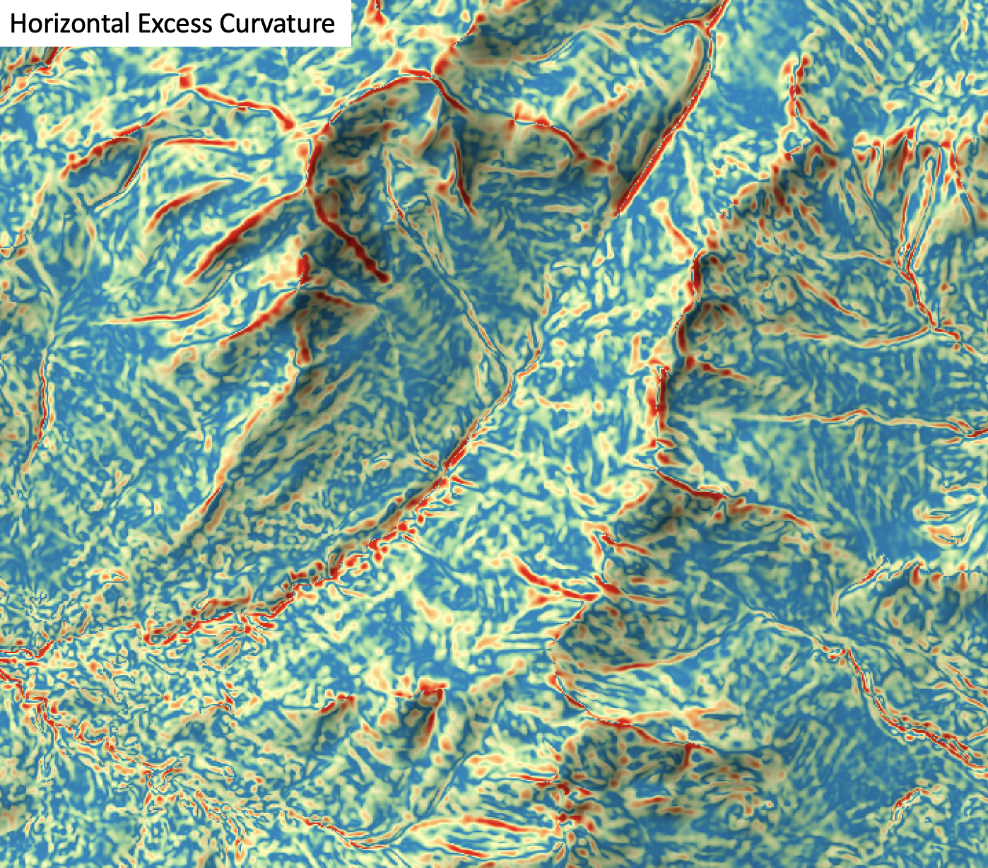
The user must specify the name of the input DEM (dem) and the output raster (output). The
The Z conversion factor (zfactor) is only important when the vertical and horizontal units are not the
same in the DEM. When this is the case, the algorithm will multiply each elevation in the DEM by the
Z Conversion Factor. Curvature values are often very small and as such the user may opt to log-transform
the output raster (log). Transforming the values applies the equation by Shary et al. (2002):
Θ' = sign(Θ) ln(1 + 10n|Θ|)
where Θ is the parameter value and n is dependent on the grid cell size.
For DEMs in projected coordinate systems, the tool uses the 3rd-order bivariate Taylor polynomial method described by Florinsky (2016). Based on a polynomial fit of the elevations within the 5x5 neighbourhood surrounding each cell, this method is considered more robust against outlier elevations (noise) than other methods. For DEMs in geographic coordinate systems (i.e. angular units), the tool uses the 3x3 polynomial fitting method for equal angle grids also described by Florinsky (2016).
References
Florinsky, I. (2016). Digital terrain analysis in soil science and geology. Academic Press.
Florinsky, I. V. (2017). An illustrated introduction to general geomorphometry. Progress in Physical Geography, 41(6), 723-752.
Shary PA (1995) Land surface in gravity points classification by a complete system of curvatures. Mathematical Geology 27: 373–390.
Shary P. A., Sharaya L. S. and Mitusov A. V. (2002) Fundamental quantitative methods of land surface analysis. Geoderma 107: 1–32.
See Also
tangential_curvature, profile_curvature, minimal_curvature, maximal_curvature, mean_curvature, gaussian_curvature
Function Signature
def horizontal_excess_curvature(self, dem: Raster, log_transform: bool = False, z_factor: float = 1.0) -> Raster: ...
hydrologic_connectivity
License Information
Use of this function requires a license for Whitebox Workflows for Python Professional (WbW-Pro). Please visit www.whiteboxgeo.com to purchase a license.
Theory
This tool calculates two indices related to hydrologic connectivity within catchments, the downslope unsaturated length (DUL) and the upslope disconnected saturated area (UDSA). Both of these hydrologic indices are based on the topographic wetness index (wetness_index), which measures the propensity for a site to be saturated to the surface, and therefore, to contribute to surface runoff. The wetness index (WI) is commonly used in hydrologic modelling, and famously in the TOPMODEL, to simulate variable source area (VSA) dynamics within catchments. The VSA is a dynamic region of surface-saturated soils within catchments that contributes fast overland flow to downslope streams during periods of precipitation. As a catchment's soil saturation deficit decreases ('wetting up'), areas with increasingly lower WI values become saturated to the surface. That is, areas of high WI are the first to become saturated and as the moisture deficit decreases, lower WI-valued cells become saturated, increasing the spatial extent of the source area. As a catchment dries out, the opposite effect occurs. The distribution of WI can therefore be used to map the spatial dyanamics of the VSA. However, the assumption in the TOPMODEL is that any rainfall over surface saturated areas will contribute to fast overland flow pathways and to stream discharge within the time step.
This method therefore implicitly assumes that all surface saturated grid cells are connected by continuously saturated areas along the downslope flow path connecting the cells to the stream. By comparison, Lane et al. (2004) proposed a modified WI, known as the network index (NI), which allowed for the modelling of disconnected, non-contributing saturated areas. The NI is essentially the downslope minimum WI. Grid cells for which WI > NI are likely to be disconnected during certain conditions from downslope streams, while similarly WI-valued cells are contributing. During these periods, any surface runoff from these cells is likely to contribute to downslope re-infilitration rather than directly to stream discharge via overland flow. This has implications for the timing and quality of stream discharge.
The DUL and UDSA indices extend the notion of the NI by mapping areas within catchments that are likely, at least during certain periods, to be sites of disconnected, non-contributing saturated areas and sites of re-infiltation respectively. These combined indices allow hydrologists to study the hydrologic connectivity and disconnectivity among areas within catchments.
The DUL (see image below) is defined for a grid cell as the number of downslope cells with a WI value lower than the current cell. Areas with non-zero DUL are likely to become fully saturated, and to contribute to overland flow, before they are directly connected to downslope areas and can contribute to stream flow. Under the appropriate catchment saturation deficit conditions, these are sites of disconnected, non-contributing saturated areas. When non-zero DUL cells are initially saturated, their precipitation excess will contribute to downslope re-infiltation, lessening the catchment's overall saturation deficit, rather than contributing to stormflow.
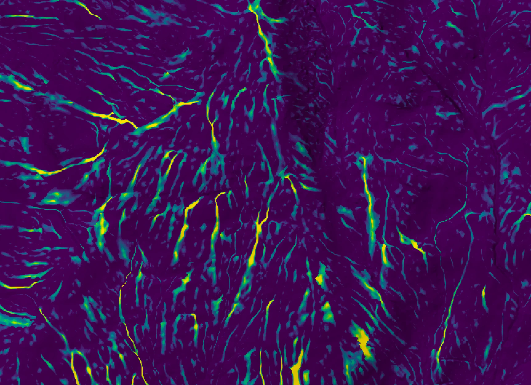
The UDSA (see image below) is defined for a grid cell as the number of upslope cells with a WI value higher than the current cell. Areas with non-zero UDSA are likely to have saturation deficits that are at least partly satisfied by local re-infiltation of overland flow from upslope areas. These non-zero UDSA cells are key sites causing the hydrologic disconnectivity of the catchment during certain conditions.
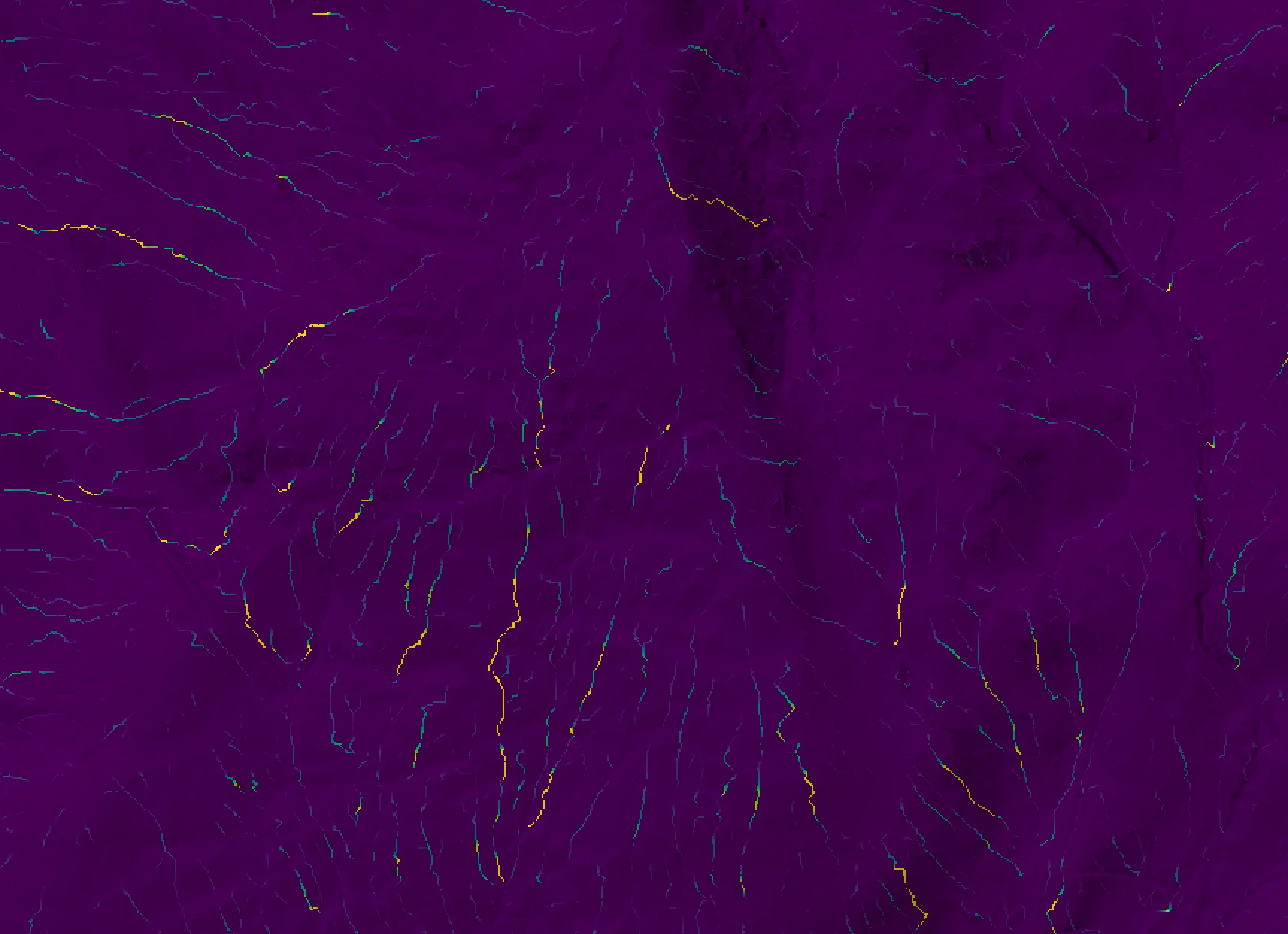
In the original Lane et al. (2004) NI paper, the authors state that the calculation of the index requires a unique, single downslope flow path for each grid cell. Therefore, the authors used the D8 single-direction flow algorithm to calculate NI. While the D8 method works well to model flow in convergent and channelized areas, it is generally recognized as a poor method for estimating WI on hillslopes, where divergent, non-chanellized flow dominates. Furthermore, the use of the D8 algorithm implied that the only way that WI can decrease downslope is for slope gradient to decrease, since specific contributing area only increases downslope with the D8 method. However, theoretically, WI may also decrease downslope due to flow dispersion, which allows for the upslope area (a surrogate for discharge) to be spread over a larger downslope dispersal area. The original NI formulation could not account for this effect.
Thus, in the implementation of the hydrologic_connectivity tool, WI is first calculated using the multiple flow-direction (MFD) algorithm described by Quinn et al. (1995), which is commonly used to estimate WI. While this implies that there are a multitude of potential flow pathways connecting each grid cell to a downstream location, in reality, if the flow path that follows the path of maximum WI issuing from a cell experiences a reduction in WI (to the point where it becomes less than the issuing cell's WI), then we can safely assume that re-infiltration occurs and the issuing cell is at times disconnected from downslope sites. Thus, after WI has been estimated using the quinn_flow_accumulation algorithm, flow directions, which are used to calculate upslope and downslope flow paths for calculating the two indices, are approximated by identifying the downslope neighbour of highest WI value for each grid cell.
Operation
The user must specify the name of the input digital elevation model (DEM; dem), and the output DUL and
UDSA rasters (output1 and output2). The DEM must have been hydrologically
corrected to remove all spurious depressions and flat areas. DEM pre-processing is usually achived using
either the breach_depressions_least_cost (also breach_depressions_least_cost) or fill_depressions tool. The
remaining two parameters are associated with the calculation of the Quinn et al. (1995) flow accumulation (quinn_flow_accumulation), used
to estimate WI. A value must be specified for the exponent parameter
(exponent), a number that controls the degree of dispersion in the flow-accumulation grid. A lower
value yields greater apparent flow dispersion across divergent hillslopes. The exponent value (h) should probably be
less than 10.0 and values between 1 and 2 are most common. The following equations are used to calculate the
portion flow (Fi) given to each neighbour, i:
Fi = Li(tanβ)p / Σi=1n[Li(tanβ)p]
p = (A / threshold + 1)h
Where Li is the contour length, and is 0.5×grid size for cardinal directions and 0.354×grid size for
diagonal directions, n = 8, and represents each of the eight neighbouring grid cells, and, A is the flow accumultation value assigned to the current grid cell, that is being
apportioned downslope. The non-dispersive, channel initiation threshold (threshold) is a flow-accumulation
value (measured in upslope grid cells, which is directly proportional to area) above which flow dispersion is
no longer permited. Grid cells with flow-accumulation values above this threshold will have their flow routed
in a manner that is similar to the D8 single-flow-direction algorithm, directing all flow towards the steepest
downslope neighbour. This is usually done under the assumption that flow dispersion, whilst appropriate on
hillslope areas, is not realistic once flow becomes channelized. Importantly, the threshold parameter sets
the spatial extent of the stream network, with lower values resulting in more extensive networks.
References
Beven K.J., Kirkby M.J., 1979. A physically-based, variable contributing area model of basin hydrology. Hydrological Sciences Bulletin 24: 43–69.
Lane, S.N., Brookes, C.J., Kirkby, M.J. and Holden, J., 2004. A network‐index‐based version of TOPMODEL for use with high‐resolution digital topographic data. Hydrological processes, 18(1), pp.191-201.
Quinn, P. F., K. J. Beven, Lamb, R. 1995. The in (a/tanβ) index: How to calculate it and how to use it within the topmodel framework. Hydrological processes 9(2): 161-182.
See Also
wetness_index, quinn_flow_accumulation
Function Signature
def hydrologic_connectivity(self, dem: Raster, exponent: float = 1.1, convergence_threshold: float = 0.0, z_factor: float = 1.0 ) -> Tuple[Raster, Raster]: ...
image_segmentation
License Information
Use of this function requires a license for Whitebox Workflows for Python Professional (WbW-Pro). Please visit www.whiteboxgeo.com to purchase a license.
Description
This tool is used to segment a mult-spectral image data set, or multi-dimensional data stack. The
algorithm is based on region-growing operations. Each of the input images are transformed into
standard scores prior to analysis. The total multi-dimensional
distance between each pixel and its eight neighbours is measured, which then serves as a priority
value for selecting potential seed pixels for the region-growing operations, with pixels exhibited the least
difference with their neighbours more likely to serve as seeds. The region-growing operations
initiate at seed pixels and grows outwards, connecting neighbouring pixels that have a multi-dimensional
distance from the seed cell that is less than a threshold value. Thus, the region-growing operations attempt
to identify contiguous, relatively homogeneous objects. The algorithm stratifies potential seed pixels into
bands, based on their total difference with their eight neighbours. The user may control the size and number
of these bands using the threshold and steps parameters respectively. Increasing the magnitude of the
threshold parameter will result in fewer mapped objects and vice versa. All pixels that are not assigned to an
object after the seeding-based region-growing operations are then clumped simply based on contiguity.
It is commonly the case that there will be a large number of very small-sized objects identified using this
approach. The user may optionally specify that objects that are less than a minimum area (expressed in pixels)
be eliminated from the final output raster. The min_area parameter must be an integer between 1 and 8. In
cleaning small objects from the output, the pixels belonging to these smaller features are assigned to the
most homogeneous neighbouring object.
The input rasters (inputs) may be bands of satellite imagery, or any other attribute, such as measures
of texture, elevation, or other topographic derivatives, such as slope. If satellite imagery is used
as inputs, it can be beneficial to pre-process the data with an edge-preserving low-pass filter, such as
the bilateral_filter and edge_preserving_mean_filter tools.
See Also
bilateral_filter, edge_preserving_mean_filter
Function Signature
def image_segmentation(self, input_rasters: List[Raster], dist_threshold: float = 0.5, num_steps: int = 10, area_threshold: int = 4) -> Raster: ...
image_slider
License Information
Use of this function requires a license for Whitebox Workflows for Python Professional (WbW-Pro). Please visit www.whiteboxgeo.com to purchase a license.
Description
This tool creates an interactive image slider from two input images (input1 and input2). An
image slider is an interactive visualization of two overlapping images, in which the user moves the
position of a slider bar to hide or reveal one of the overlapping images. The output (output)
is an HTML file. Each of the two input images may be rendered in one of several available palettes.
If the input image is a colour composite image, no palette is required. Labels may also be optionally
associated with each of the images, displayed in the upper left and right corners. The user must also
specify the image height (height) in the output file. Note that the output is simply HTML, CSS, and
javascript code, which can be readily embedded in other documents.
The following is an example of what the output of this tool looks like. Click the image for an interactive example.
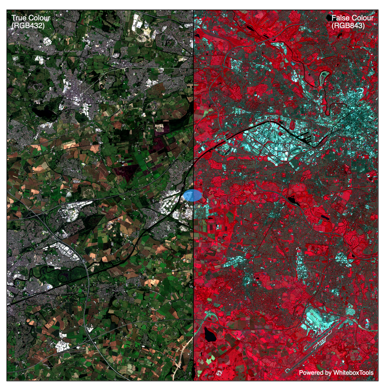
Function Signature
def image_slider(self, left_raster: Raster, right_raster: Raster, output_html_file: str, left_palette: WbPalette = WbPalette.Grey, left_reverse_palette: bool = False, left_label: str = "", right_palette: WbPalette = WbPalette.Grey, right_reverse_palette: bool = False, right_label: str = "", image_height: int = 600) -> None: ...
improved_ground_point_filter
Use of this function requires a license for Whitebox Workflows for Python Professional (WbW-Pro). Please visit www.whiteboxgeo.com to purchase a license.
This function provides a faster alternative to the lidar_ground_point_filter algorithm, provided in the free
version of Whitebox Workflows, for the extraction of ground points from within a LiDAR point cloud. The algorithm
works by placing a grid overtop of the point cloud of a specified resolution (block_size, in xy-units) and identifying the
subset of lidar points associated with the lowest position in each block. A raster surface is then created by
TINing these points. The surface is further processed by removing any off-terrain objects (OTOs), including buildings
smaller than the max_building_size parameter (xy-units). Removing OTOs also requires the user to specify the value of
a slope_threshold, in degrees. Finally, the algorithm then extracts all of the points in the input LiDAR point cloud
(input) that are within a specified absolute vertical distance (elev_threshold) of this surface model.
Conceptually, this method of ground-point filtering is somewhat similar in concept to the cloth-simulation approach of
Zhang et al. (2016). The difference is that the cloth is first fitted to the minimum surface with infinite flexibility
and then the rigidity of the cloth is subsequently increased, via the identification and removal of OTOs from the minimal
surface. The slope_threshold parameter effectively controls the eventual rigidity of the fitted surface.
By default, the tool will return a point cloud containing only the subset of points in the input dataset that coincide
with the idenfitied ground points. Setting the classify parameter to True modifies this behaviour such that the output
point cloud will contain all of the points within the input dataset, but will have the classification value of identified
ground points set to '2' (i.e., the ground class value) and all other points will be set to '1' (i.e., the unclassified
class value). By setting the preserve_classes paramter to True, all non-ground points in the output cloud will have
the same classes as the corresponding point class values in the input dataset.
Compared with the lidar_ground_point_filter algorithm, the improved_ground_point_filter algorithm is generally far faster and is able to more effectively remove points associated with larger buildings. Removing large buildings from point clouds with the lidar_ground_point_filter algorithm requires use of very large search distances, which slows the operation considerably.
As a comparison of the two available methods, one test tile of LiDAR containing numerous large buildings and abundant vegetation required 600.5 seconds to process on the test system using the lidar_ground_point_filter algorithm (removing all but the largest buildings) and 9.8 seconds to process using the improved_ground_point_filter algorithm (with complete building removal), i.e., 61x faster.
The original test LiDAR tile, containing abundant vegetation and buildings:
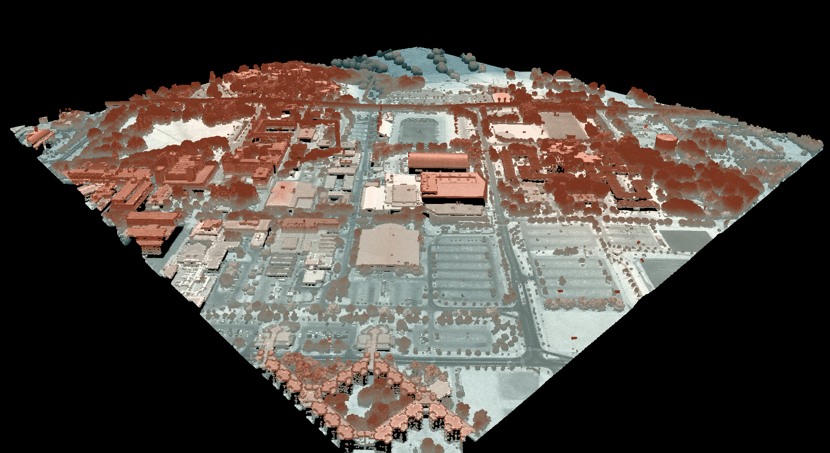
The result of applying the lidar_ground_point_filter function, with a search radius of 25 m and max inter-point slope of 15 degrees:
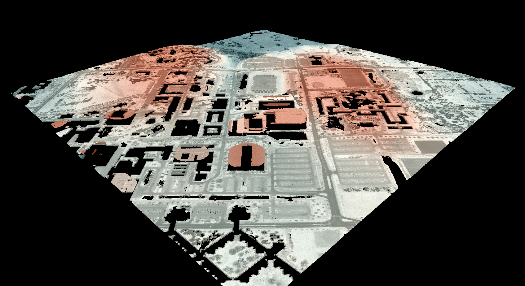
The result of applying the improved_ground_point_filter method, with block_size = 1.0 m, max_building_size = 150.0 m,
slope_threshold = 15.0 degrees, and elev_threshold = 0.15 m:
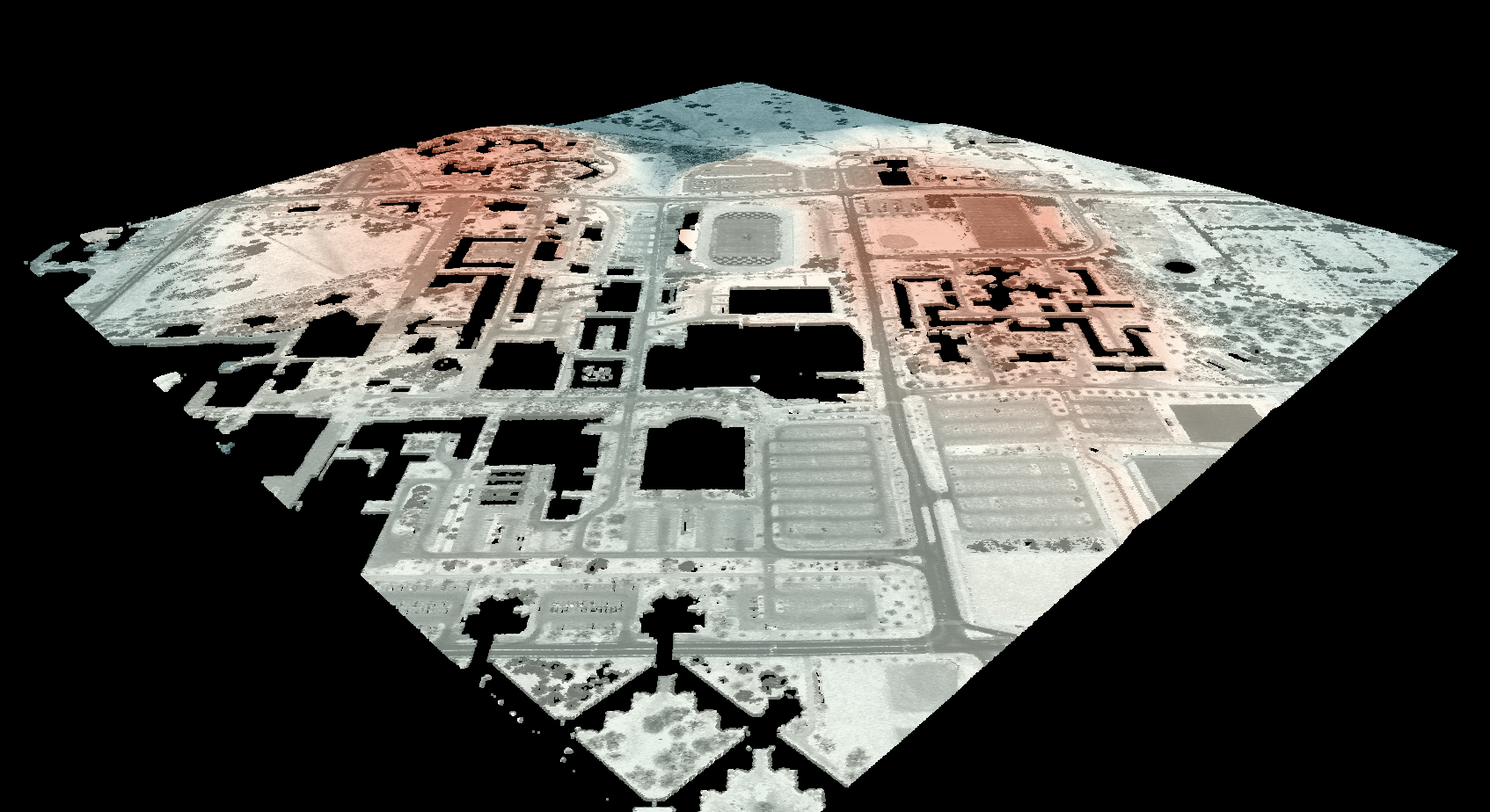
References:
Zhang, W., Qi, J., Wan, P., Wang, H., Xie, D., Wang, X., & Yan, G. (2016). An easy-to-use airborne LiDAR data filtering method based on cloth simulation. Remote sensing, 8(6), 501.
See Also:
Function Signature
def improved_ground_point_filter(self, input: Lidar, block_size = 1.0, max_building_size = 150.0, slope_threshold = 15.0, elev_threshold = 0.15, , classify = False, preserve_classes = False) -> Lidar: ...
inverse_pca
License Information
Use of this function requires a license for Whitebox Workflows for Python Professional (WbW-Pro). Please visit www.whiteboxgeo.com to purchase a license.
Description
This tool takes a two or more component images (inputs), and the
principal component analysis (PCA)
report derived using the principal_component_analysis tool, and performs the inverse PCA transform to
derive the original series of input images. This inverse transform is frequently performed to reduce
noise within a multi-spectral image data set. With a typical PCA transform, high-frequency noise will
commonly map onto the higher component images. By excluding one or more higher-valued component
images from the input component list, the inverse transform can produce a set of images in the
original coordinate system that exclude the information contained within component images excluded
from the input list. Note that the number of output images will also equal the number of original
images input to the principal_component_analysis tool. The output images will be named automatically
with a "inv_PCA_image" suffix.
See Also
Function Signature
def inverse_pca(self, rasters: List[Raster], pca_report_file: str) -> List[Raster]: ...
knn_classification
License Information
Use of this function requires a license for Whitebox Workflows for Python Professional (WbW-Pro). Please visit www.whiteboxgeo.com to purchase a license.
Description
This tool performs a supervised k-nearest neighbour (k-NN) classification
using multiple predictor rasters (inputs), or features, and training data (training). It can be used to model
the spatial distribution of class data, such as land-cover type, soil class, or vegetation type.
The training data take
the form of an input vector Shapefile containing a set of points or polygons, for which the known
class information is contained within a field (field) of the attribute table. Each grid cell defines
a stack of feature values (one value for each input raster), which serves as a point within the
multi-dimensional feature space. The algorithm works by identifying a user-defined number (k, -k) of
feature-space neighbours from the training set for each grid cell. The class that is then assigned to
the grid cell in the output raster (output) is then determined as the most common class among the
set of neighbours. Note that the knn_regression tool can be used to apply the k-NN method to the modelling
of continuous data.
The user has the option to clip the training set data (clip). When this option is selected, each training pixel for which the estimated class value, based on the k-NN procedure, is not equal to the known class value, is removed from the training set before proceeding with labelling all grid cells. This has the effect of removing outlier points within the training set and often improves the overall classification accuracy.
The tool splits the training data into two sets, one for training the classifier and one for testing
the classification. These test data are used to calculate the overall accuracy and Cohen's kappa
index of agreement, as well as to estimate the variable importance. The test_proportion parameter
is used to set the proportion of the input training data used in model testing. For example, if
test_proportion = 0.2, 20% of the training data will be set aside for testing, and this subset
will be selected randomly. As a result of this random selection of test data, the tool behaves stochastically,
and will result in a different model each time it is run.
Note that the output image parameter (output) is optional. When unspecified, the tool will simply
report the model accuracy statistics and variable importance, allowing the user to experiment with different parameter
settings and input predictor raster combinations to optimize the model before applying it to classify
the whole image data set.
Like all supervised classification methods, this technique relies heavily on proper selection of training data. Training sites are exemplar areas/points of known and representative class value (e.g. land cover type). The algorithm determines the feature signatures of the pixels within each training area. In selecting training sites, care should be taken to ensure that they cover the full range of variability within each class. Otherwise the classification accuracy will be impacted. If possible, multiple training sites should be selected for each class. It is also advisable to avoid areas near the edges of class objects (e.g. land-cover patches), where mixed pixels may impact the purity of training site values.
After selecting training sites, the feature value distributions of each class type can be assessed using the evaluate_training_sites tool. In particular, the distribution of class values should ideally be non-overlapping in at least one feature dimension.
The k-NN algorithm is based on the calculation of distances in multi-dimensional space. Feature scaling is
essential to the application of k-NN modelling, especially when the ranges of the features are different, for
example, if they are measured in different units. Without scaling, features with larger ranges will have
greater influence in computing the distances between points. The tool offers three options for feature-scaling (scaling),
including 'None', 'Normalize', and 'Standardize'. Normalization simply rescales each of the features onto
a 0-1 range. This is a good option for most applications, but it is highly sensitive to outliers because
it is determined by the range of the minimum and maximum values. Standardization
rescales predictors using their means and standard deviations, transforming the data into z-scores. This
is a better option than normalization when you know that the data contain outlier values; however, it does
does assume that the feature data are somewhat normally distributed, or are at least symmetrical in
distribution.
Because the k-NN algorithm calculates distances in feature-space, like many other related algorithms, it suffers from the curse of dimensionality. Distances become less meaningful in high-dimensional space because the vastness of these spaces means that distances between points are less significant (more similar). As such, if the predictor list includes insignificant or highly correlated variables, it is advisable to exclude these features during the model-building phase, or to use a dimension reduction technique such as principal_component_analysis to transform the features into a smaller set of uncorrelated predictors.
For a video tutorial on how to use the knn_classification tool, see this YouTube video.
Memory Usage
The peak memory usage of this tool is approximately 8 bytes per grid cell × # predictors.
See Also
knn_regression, random_forest_classification, svm_classification, parallelepiped_classification, evaluate_training_sites
Function Signature
def knn_classification(self, input_rasters: List[Raster], training_data: Vector, class_field_name: str, scaling_method: str = "none", k: int = 5, test_proportion: float = 0.2, use_clipping: bool = False, create_output: bool = False) -> Optional[Raster]: ...
knn_regression
License Information
Use of this function requires a license for Whitebox Workflows for Python Professional (WbW-Pro). Please visit www.whiteboxgeo.com to purchase a license.
Description
This tool performs a supervised k-nearest neighbour (k-NN) regression analysis
using multiple predictor rasters (inputs), or features, and training data (training). It can be used to model
the spatial distribution of continuous data, such as soil properties (e.g. percent sand/silt/clay).
The training data take the form of an input vector Shapefile containing a set of points, for which the known
outcome information is contained within a field (field) of the attribute table. Each grid cell defines
a stack of feature values (one value for each input raster), which serves as a point within the
multi-dimensional feature space. The algorithm works by identifying a user-defined number (k, -k) of
feature-space neighbours from the training set for each grid cell. The value that is then assigned to
the grid cell in the output raster (output) is then determined as the mean of the outcome variable
among the set of neighbours. The user may optionally choose to weight neighbour outcome values in
the averaging calculation, with weights determined by the inverse distance function (weight). Note
that the knn_classification tool can be used to apply the k-NN method to the modelling of categorical
data.
The tool splits the training data into two sets, one for training the model and one for testing
the prediction. These test data are used to calculate the regression accuracy statistics, as
well as to estimate the variable importance. The test_proportion parameter
is used to set the proportion of the input training data used in model testing. For example, if
test_proportion = 0.2, 20% of the training data will be set aside for testing, and this subset
will be selected randomly. As a result of this random selection of test data, the tool behaves stochastically,
and will result in a different model each time it is run.
Note that the output image parameter (output) is optional. When unspecified, the tool will simply
report the model accuracy statistics and variable importance, allowing the user to experiment with different parameter
settings and input predictor raster combinations to optimize the model before applying it to model the
outcome variable across the whole region defined by image data set.
The k-NN algorithm is based on the calculation of distances in multi-dimensional space. Feature scaling is
essential to the application of k-NN modelling, especially when the ranges of the features are different, for
example, if they are measured in different units. Without scaling, features with larger ranges will have
greater influence in computing the distances between points. The tool offers three options for feature-scaling (scaling),
including 'None', 'Normalize', and 'Standardize'. Normalization simply rescales each of the features onto
a 0-1 range. This is a good option for most applications, but it is highly sensitive to outliers because
it is determined by the range of the minimum and maximum values. Standardization
rescales predictors using their means and standard deviations, transforming the data into z-scores. This
is a better option than normalization when you know that the data contain outlier values; however, it does
does assume that the feature data are somewhat normally distributed, or are at least symmetrical in
distribution.
Because the k-NN algorithm calculates distances in feature-space, like many other related algorithms, it suffers from the curse of dimensionality. Distances become less meaningful in high-dimensional space because the vastness of these spaces means that distances between points are less significant (more similar). As such, if the predictor list includes insignificant or highly correlated variables, it is advisable to exclude these features during the model-building phase, or to use a dimension reduction technique such as principal_component_analysis to transform the features into a smaller set of uncorrelated predictors.
Memory Usage
The peak memory usage of this tool is approximately 8 bytes per grid cell × # predictors.
See Also
knn_classification, random_forest_regression, svm_regression, principal_component_analysis
Function Signature
def knn_regression(self, input_rasters: List[Raster], training_data: Vector, field_name: str, scaling_method: str = "none", k: int = 5, distance_weighting: bool = False, test_proportion: float = 0.2, create_output: bool = False) -> Optional[Raster]: ...
lidar_contour
License Information
Use of this function requires a license for Whitebox Workflows for Python Professional (WbW-Pro). Please visit www.whiteboxgeo.com to purchase a license.
Description
This tool can be used to create a contour (i.e. isolines
of elevation values) vector coverage from an input LiDAR points data set (input). The tool works by first
creating a triangulation of the input LiDAR points. The user must specify the
contour interval (interval), or vertical spacing between contour lines. The smooth parameter can
be used to increase or decrease the degree to which contours are smoothed. This parameter should be an
odd integer value (0, 1, 3, 5...), with 0 indicating no smoothing. The tool can interpolate
contours based on the LiDAR point elevation values, intensity data, or the user data field (parameter),
with 'elevation' as the default parameter. LiDAR points may be excluded from the contouring process based
on a number of criteria, including their return value (returns, which may be 'all', 'last', 'first'),
their class value (exclude_cls), and whether they fall outside of a user-specified elevation range
(minz and maxz). The optional max_triangle_edge_length parameter can be used to exclude
the output of contours within areas that are sparsely populated areas of the data set, where the triangles
formed by the Delaunay triangulation are too large. This is often the case within bodies of water; long
and narrow triangular facets can also occur within the concave portions of the hull, or polygon enclosing,
the points, when the data have an irregular shaped extent. Setting this parameter can help alleviate the
problem of contouring beyond the data footprint.
Like many of the LiDAR tools, both the input and output parameters are optional. If these
parameters are not specified by the user, the tool will search for all LAS files contained within the
current WhiteboxTools working directory. This feature can be useful when you need to contour a large
number of LiDAR tiles. This batch processing mode enables the tool to enable parallel data processing,
which can significantly improve the efficiency of data conversion for datasets with many LiDAR tiles.
When run in this batch mode, the output file (output) also need not be specified; the tool will
instead create an output file with the same name as each input LiDAR file, but with the .shp extension.
It is important to note that contouring is better suited to well-defined surfaces (e.g. the ground surface or building heights), rather than volume features, such as vegetation, which tend to produce extremely complex contour sets. It is advisable to use this tool with last-returns and/or ground-classified point returns. If the input data set does not contain ground classification, consider pre-processing with the lidar_ground_point_filter tool.
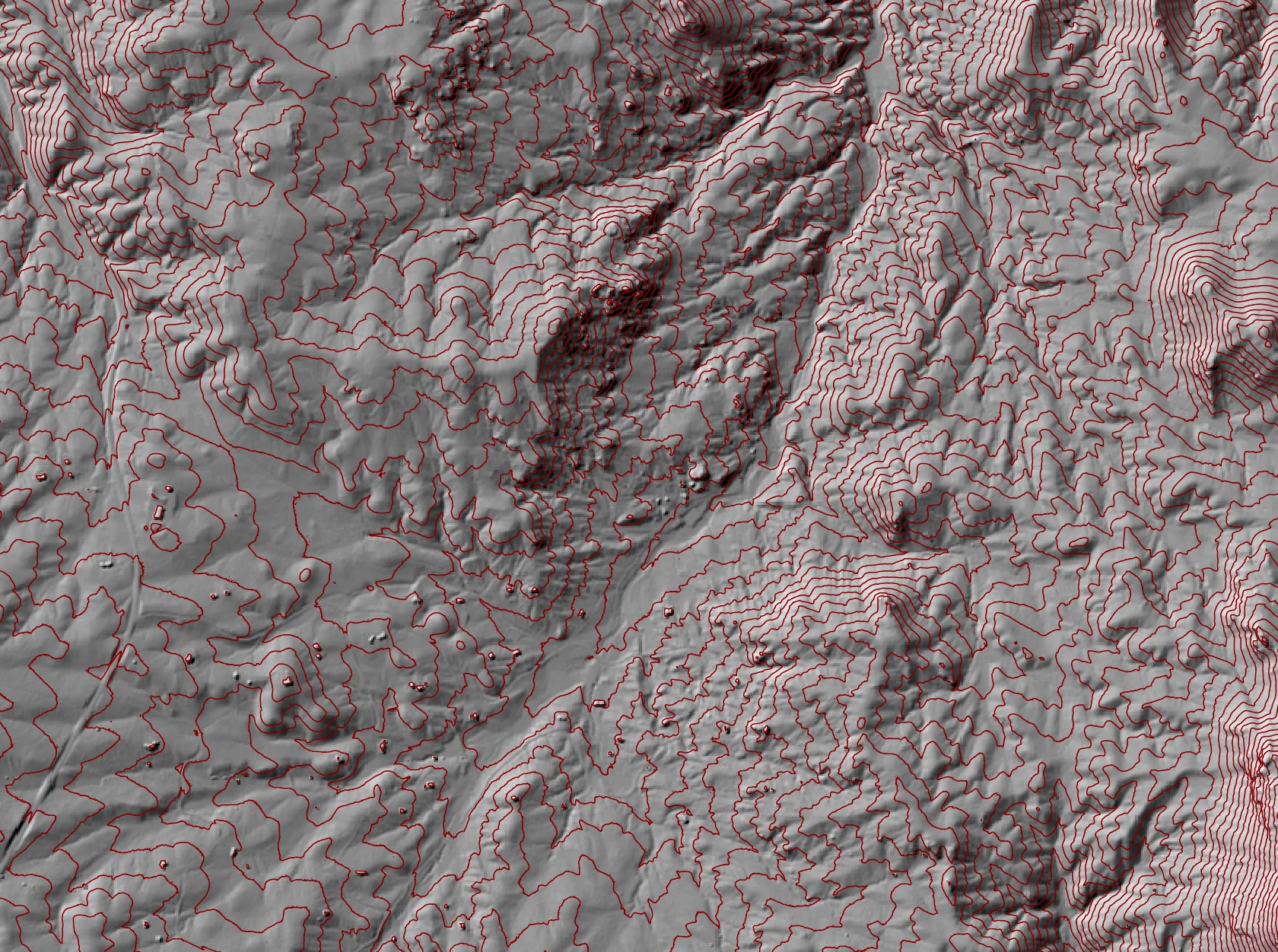
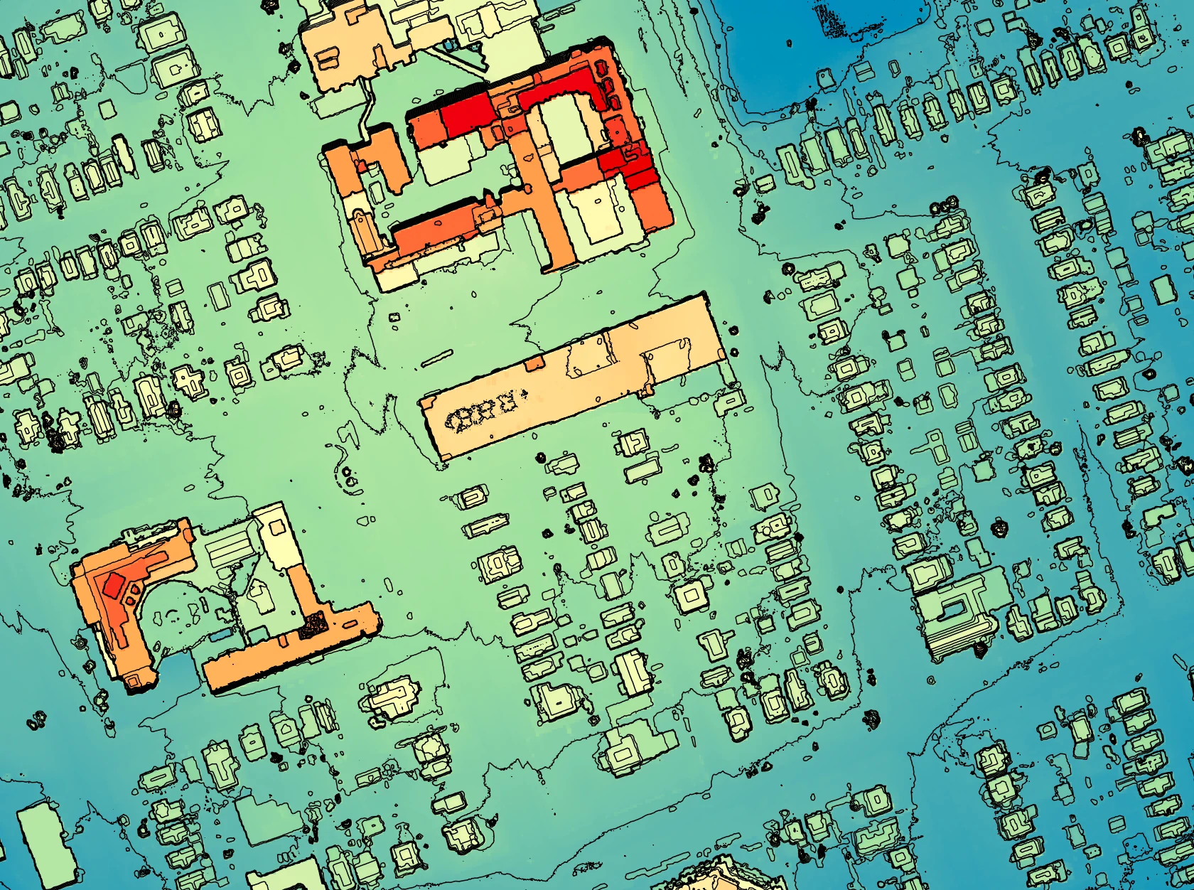
See Also
contours_from_points, contours_from_raster, lidar_ground_point_filter
Function Signature
def lidar_contour(self, input_lidar: Optional[Lidar], contour_interval: float = 10.0, base_contour: float = 0.0, smooth: int = 5, interpolation_parameter: str = "elevation", returns_included: str = "all", excluded_classes: Optional[List[int]] = None, min_elev: float = float('-inf'), max_elev: float = float('inf'), tile_overlap: float = 0.0, max_triangle_edge_length: float = float('inf')) -> Optional[Vector]: ...
lidar_eigenvalue_features
License Information
Use of this function requires a license for Whitebox Workflows for Python Professional (WbW-Pro). Please visit www.whiteboxgeo.com to purchase a license.
Description
This tool can be used to measure eigenvalue-based features that describe the characteristics of the local
neighbourhood surrounding each point in an input LiDAR file (input). These features can then be used in
point classification applications, or as the basis for point filtering (filter_lidar) or modifying point
properties (modify_lidar).
The algorithm begins by using the x, y, z coordinates of the points within a local spherical neighbourhood to calculate a covariance matrix. The three eigenvalues λ1, λ2, λ3 are then derived from the covariance matrix decomposition such that λ1 > λ2 > λ3. The eigenvalues are then used to describe the extent to which the neighbouring points can be characterized by a linear, planar, or volumetric distribution, by calculating the following three features:
linearity = (λ1 - λ2) / λ1
planarity = (λ2 - λ3) / λ1
sphericity = λ3 / λ1
In the case of a neighbourhood containing a 1-dimensional line, the first of the three components will possess most of data variance, with very little contained within λ2 and λ3, and linearity will be nearly equal to 1.0. If the local neighbourhood contains a 2-dimensional plane, the first two components will possess most of the variance, with little variance within λ3, and planarity will be nearly equal to 1.0. Lastly, in the case of a 3-dimensional, random volumetric point distribution, each of the three components will be nearly equal in magnitude and sphericity will be nearly equal to 1.0.
Researchers in the field of LiDAR point classification also frequently define two additional eigenvalue-based features, the omnivariance (low values correspond to planar and linear regions and higher values occur for areas with a volumetric point distribution, such as vegetation), and the eigentropy, which is related to the Shannon entropy and is a measure of the unpredictability of the distribution of points in the neighbourhood:
omnivariance = (λ1 ⋅ λ2 ⋅ λ3)1/3
eigentropy = -e1 ⋅ lne1 - e2 ⋅ lne2 - e3 ⋅ lne3
where e1, e2, and e3 are the normalized eigenvalues.
In addition to the eigenvalues, the eigendecomposition of the symmetric covariance matrix also yields the three eigenvectors, which describe the transformation coefficients of the principal components. The first two eigenvectors represent the basis of the plane resulting from the orthogonal regression analysis, while the third eigenvector represents the plane normal. From this normal, it is possible to calculate the slope of the plane, as well as the orthogonal distance between each point and the neighbourhood fitted plane, i.e. the point residual.
This tool outputs a binary file (*.eigen; output) that contains a total of 10 features for each
point in the input file, including the point_num (for reference), lambda1, lambda2, lambda3, linearity,
planarity, sphericity, omnivariance, eigentropy, slope, and residual. Users should bear in mind
that most of these features describe the properties of the distribution of points within a spherical neighbourhood
surrounding each point in the input file, rather than a characteristic of the point itself. The only one
of the ten features that is a point property is the residual. Points for which the planarity value is high and the
residual value is low may be assumed to be part of the plane that dominate the structure of their neighbourhoods.
In addition to the binary data *.eigen file, the tool will also output a sidecar file,
with a *.eigen.json extension, which describes the structure of the raw binary data file.
Local neighbourhoods are spherical in shape and the size of each neighbourhood is characterized by the
num_neighbours and radius parameters. If the optional num_neighbours parameter is specified,
the size of the neighbourhood will vary by point, increasing or decreasing to encompass the specified number
of neighbours (notice that this value does not include the point itself). If the optional radius parameter
is specified in addition to a number of neighbours, the specified radius value will serve as a upper-bound
and neighbouring points that are beyond this radial distance to the centre point will be excluded. If a radius
search distance is specified but the num_neighbours parameter is not, then a constant search distance will
be used for each point in the input file, resulting in varying number of points within local neighbourhoods,
depending on local point densities. If point density varies significantly in the input file, then use of the
num_neighbours parameter may be advisable. Notice that at least one of the two parameters must be specified.
In cases where the number of neighbouring points is fewer than eight, each of the output feature values will
be set to 0.0.
Note that if the user does not specify the optional input LiDAR file, the tool will search for all valid LiDAR (*.las, *.laz, *.zlidar) files contained within the current working directory. This feature can be useful for processing a large number of LiDAR files in batch mode.
The binary data file (*.eigen) can be used directly by the filter_lidar and modify_lidar tools, and will
be automatically read by the tools when the *.eigen and *.eigen.json files are present in the same
folder as the accompanying source LiDAR file. This allows users to apply
data filters, or to modify point properties, using these point neighbourhood features. For example, the
statement, rgb=(int(linearity*255), int(planarity*255), int(sphericity*255)), used with the modify_lidar
tool, can render the point RGB colour values based on some of the eigenvalue features, allowing users to
visually identify linear features (red), planar features (green), and volumetric regions (blue).
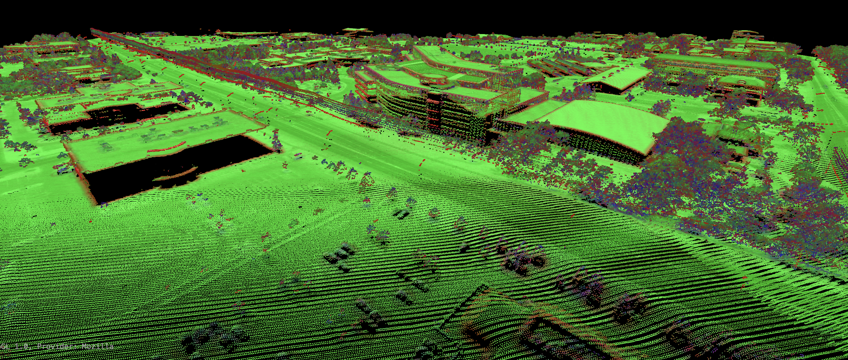
Additionally, these features data can also be readily incorporated into a Python-based point analysis or classification. As an example, the following script reads in a *.eigen binary data file for direct manipulation and analysis:
import numpy as np

dt = np.dtype([
('point_num', '<u8'),
('lambda1', '<f4'),
('lambda2', '<f4'),
('lambda3', '<f4'),
('linearity', '<f4'),
('planarity', '<f4'),
('sphericity', '<f4'),
('omnivariance', '<f4'),
('eigentropy', '<f4'),
('slope', '<f4'),
('resid', '<f4')
])

with open('/Users/johnlindsay/Documents/data/aaa2.eigen', 'rb') as f:
b = f.read()

pt_features = np.frombuffer(b, dt)

# Print the first 100 point features to demonstrate
for i in range(100):
print(f"{pt_features['point_num'][i]} {pt_features['linearity'][i]} {pt_features['planarity'][i]} {pt_features['sphericity'][i]}")


print("Done!")
References
Chehata, N., Guo, L., & Mallet, C. (2009). Airborne lidar feature selection for urban classification using random forests. In Laser Scanning IAPRS, Vol. XXXVIII, Part 3/W8 – Paris, France, September 1-2, 2009.
Gross, H., Jutzi, B., & Thoennessen, U. (2007). Segmentation of tree regions using data of a full-waveform laser. International Archives of Photogrammetry, Remote Sensing and Spatial Information Sciences, 36(part 3), W49A.
Niemeyer, J., Mallet, C., Rottensteiner, F., & Sörgel, U. (2012). Conditional Random Fields for the Classification of LIDAR Point Clouds. In XXII ISPRS Congress at Melbourne, ISPRS Annals of the Photogrammetry, Remote Sensing and Spatial Information Sciences (Vol. 3).
West, K. F., Webb, B. N., Lersch, J. R., Pothier, S., Triscari, J. M., & Iverson, A. E. (2004). Context-driven automated target detection in 3D data. In Automatic Target Recognition XIV (Vol. 5426, pp. 133-143). SPIE.
See Also
filter_lidar, modify_lidar, sort_lidar, split_lidar
Function Signature
def lidar_eigenvalue_features(self, input_lidar: Optional[Lidar], num_neighbours: Optional[int], search_radius: Optional[float]) -> None: ...
lidar_point_return_analysis
License Information
Use of this function requires a license for Whitebox Workflows for Python Professional (WbW-Pro). Please visit www.whiteboxgeo.com to purchase a license.
Description
This performs a quality control check on the return values of points in a LiDAR file. In particular, the tool will search for missing point returns, duplicate point returns, and points for which the return number (r) is larger than the encoded number of returns (n), all of which may be indicative of processing or encoding errors in the input file.
The user must specify the name of the input LiDAR file (input), and may optionally specify an output
LiDAR file (output). If no output file is specified, only the text report is generated by the tool. If
an output is specified, the tool will create an output LiDAR file for which missing returns are assigned
class 13, duplicate returns are assigned class 14, points that are both, part of a missing series and are
duplicate returns, are classed 15, and all other non-problemmatic points are assigned class 1. Note, those
points designated as missing in the output image are clearly not so much missing as they are part of a
sequence of points that contain missing returns. Missing points are apparent when the first point in a series
does not have r = 1, when the last point does not have r = n, or the series is non-sequential (e.g.
1/3, 3/3, but no 2/3). This condition may occur because returns are split between tiles. However, when
sequences with missing points are not located near the edges of tiles, it is usually an indication that either
point filtering has taken place during pre-processing or that there is been some kind of processing or encoding
error.
Duplicate points are defined as points that share the same time, scanner channel, r, and n. Note that these points may have different x, y, z coordinates. Duplicate points are always an indication of a processing or encoding error. For example, it may indicate that the scanner channel information from a multi-channel LiDAR sensor has not been encoded when creating the file or has been lost.
No point should have r > n. This always indicates some kind of processing or encoding error when it occurs.
The following is a sample output report generated by this tool:
***************************************
* Welcome to LidarPointReturnAnalysis *
***************************************
The Global Encoding for this file indicates that
the point returns are not synthetic.

Missing Returns:
2441636 (16.336 percent) points are missing

| r | n | Missing Pts |
|---|---|-------------|
| 1 | 2 |     1127770 |
| 2 | 2 |         817 |
| 1 | 3 |      823240 |
| 2 | 3 |         569 |
| 3 | 3 |         718 |
| 1 | 4 |      285695 |
| 2 | 4 |      142890 |
| 3 | 4 |         142 |
| 4 | 4 |         213 |
| 1 | 5 |       29772 |
| 2 | 5 |       19848 |
| 3 | 5 |        9928 |
| 4 | 5 |          18 |
| 5 | 5 |          16 |


Duplicate Returns:
4311021 (28.844 percent) points are duplicates

| r | n | Duplicates |
|---|---|------------|
| 1 | 1 |    2707083 |
| 1 | 2 |     332028 |
| 2 | 2 |     663717 |
| 1 | 3 |      70619 |
| 2 | 3 |     211834 |
| 3 | 3 |     282348 |
| 1 | 4 |       2856 |
| 2 | 4 |       8568 |
| 3 | 4 |      14280 |
| 4 | 4 |      17136 |
| 1 | 5 |         23 |
| 2 | 5 |         69 |
| 3 | 5 |        115 |
| 4 | 5 |        161 |
| 5 | 5 |        184 |


Return Greater Than Num. Returns:
0 (0.000 percent) points have r > n

Writing output LAS file...
Complete!
Elapsed Time (including I/O): 1.959s
Function Signature
def lidar_point_return_analysis(self, input: Lidar, create_output: bool = False) -> Optional[Lidar]: ...
lidar_sibson_interpolation
License Information
Use of this function requires a license for Whitebox Workflows for Python Professional (WbW-Pro). Please visit www.whiteboxgeo.com to purchase a license.
Description
This tool interpolates LiDAR files using Sibson's interpolation method, sometimes referred to as natural-neighbour interpolation (not to be confused with nearest-neighbour interpolation, lidar_nearest_neighbour_gridding). Sibon's method is based on assigning weight to points for which inserting a grid point would result in captured areas of the Voronoi tessellation of the input point set. The larger the captured area, the higher the weight assigned to the associated point. One of the main advantages of this natural neighbour approach to interpolation over similar techniques, such as inverse-distance weighting (IDW lidar_idw_interpolation), is that there is no need to specify a search distance or other interpolation weighting parameters. Sibson's approach frequently provides a very suitable interpolation for LiDAR data. The method requires the calculation of a Delaunay triangulation, from which the Voronoi tessellation is calculated.
The user must specify the value of the IDW weight parameter (weight). The output grid can be based on any of the
stored LiDAR point parameters (parameter), including elevation (in which case the output grid is a digital
elevation model, DEM), intensity, class, return number, number of returns, scan angle values, and user data
values. Similarly, the user may specify which point return values (returns) to include in the interpolation,
including all points, last returns (including single return points), and first returns (including single return
points).
The user must specify the grid resolution of the output raster (resolution), and optionally, the name of the
input LiDAR file (input) and output raster (output). Note that if an input LiDAR file (input) is not
specified by the user, the tool will search for all valid LiDAR (*.las, *.laz, *.zlidar) files contained within the current
working directory. This feature can be useful when you need to interpolate a DEM for a large number of LiDAR
files. This batch processing mode enables the tool to include a small buffer of points extending into adjacent
tiles when interpolating an individual file. This can significantly reduce edge-effects when the output tiles are
later mosaicked together. When run in this batch mode, the output file (output) also need not be specified;
the tool will instead create an output file with the same name as each input LiDAR file, but with the .tif
extension. This can provide a very efficient means for processing extremely large LiDAR data sets.
Users may excluded points from the interpolation based on point classification values, which follow the LAS
classification scheme. Excluded classes are specified using the exclude_cls parameter. For example,
to exclude all vegetation and building classified points from the interpolation, use --exclude_cls='3,4,5,6'.
Users may also exclude points from the interpolation if they fall below or above the minimum (minz) or
maximum (maxz) thresholds respectively. This can be a useful means of excluding anomalously high or low
points. Note that points that are classified as low points (LAS class 7) or high noise (LAS class 18) are
automatically excluded from the interpolation operation.
See Also
lidar_tin_gridding, lidar_nearest_neighbour_gridding, lidar_idw_interpolation
Function Signature
def lidar_sibson_interpolation(self, input_lidar: Optional[Lidar], interpolation_parameter: str = "elevation", resolution: float = 1.0, returns_included: str = "all", excluded_classes: Optional[List[int]] = None, min_elev: float = float('-inf'), max_elev: float = float('inf')) -> Optional[Raster]: ...
local_hypsometric_analysis
License Information
Use of this function requires a license for Whitebox Workflows for Python Professional (WbW-Pro). Please visit www.whiteboxgeo.com to purchase a license.
Description
This tool calculates the hypsometric integral from the elevation distribution contained within the
local neighbourhood surrounding each grid cell in an input (input) DEM. The hyspometric integral (HI) is
the area under the hypsometric curve, which is a plot that relates elevation and area. This plot
is a cumulative distribution function with elevation expressed as a proportion of maximum elevation and
area expressed as the proportion of the area above. Hypsometry, or area-altitude analysis, is commonly
used by geomorphologists and geologists to characterize the erosional history of drainage basins. The
HI, ranging between 0 and 1, expresses the volume of land that lies above the lowest point within an
area, and thus has not been eroded. Relatively low HI values are indicative of more strongly eroded
surfaces.
Some researchers (e.g. Pérez‐Peña et al., 2009) have demonstrated the usefulness of applying hypsometry
in a spatially distributed fashion, rather than aggregated by basins, as it is typically applied. While
Pérez‐Peña et al. (2009) characterized spatial distributions of HI using coarse grids overlayed overtop
a digital elevation model (DEM), this tool uses a filter-based approach instead. Each grid cell in the
input DEM (input) has an individual HI calculation based on the elevation distribution within a
moving kernel. HI values are calculated using the elevation-relief ratio method described by Pike and
Wilson (1971).
In actuality, the tool uses a multi-scale approach, much like many of the other tools within the Geomorphometric Analysis toolbox (e.g. max_elevation_deviation, multiscale_std_dev_normals), such that the neighbourhood size is varied according to a range defined by user-specified input parameters. The HI that is reported within each grid cell in the output raster is the minimum HI value measured for each of the tested scales, defined by lower (rL) and upper (rU) ranges.
HImin=min{HI(r):r=rL...rU},
In this way, it represents a heterogenous, locally scale optimized map of HI distributions. A nonlinear scale sampling interval is used by this tool to ensure that the scale sampling density is higher for short scale ranges, where there is often greater variability in HI values, and coarser at longer tested scales, such that:
ri = rL + [step × (i - rL)]p
Where ri is the filter radius for step i and p is the nonlinear scaling factor (step_nonlinearity)
and a step size (step) of step.
There are two outputs generated from this tool, including the HImin raster (out_mag)
and the rmin scale raster (out_scale).
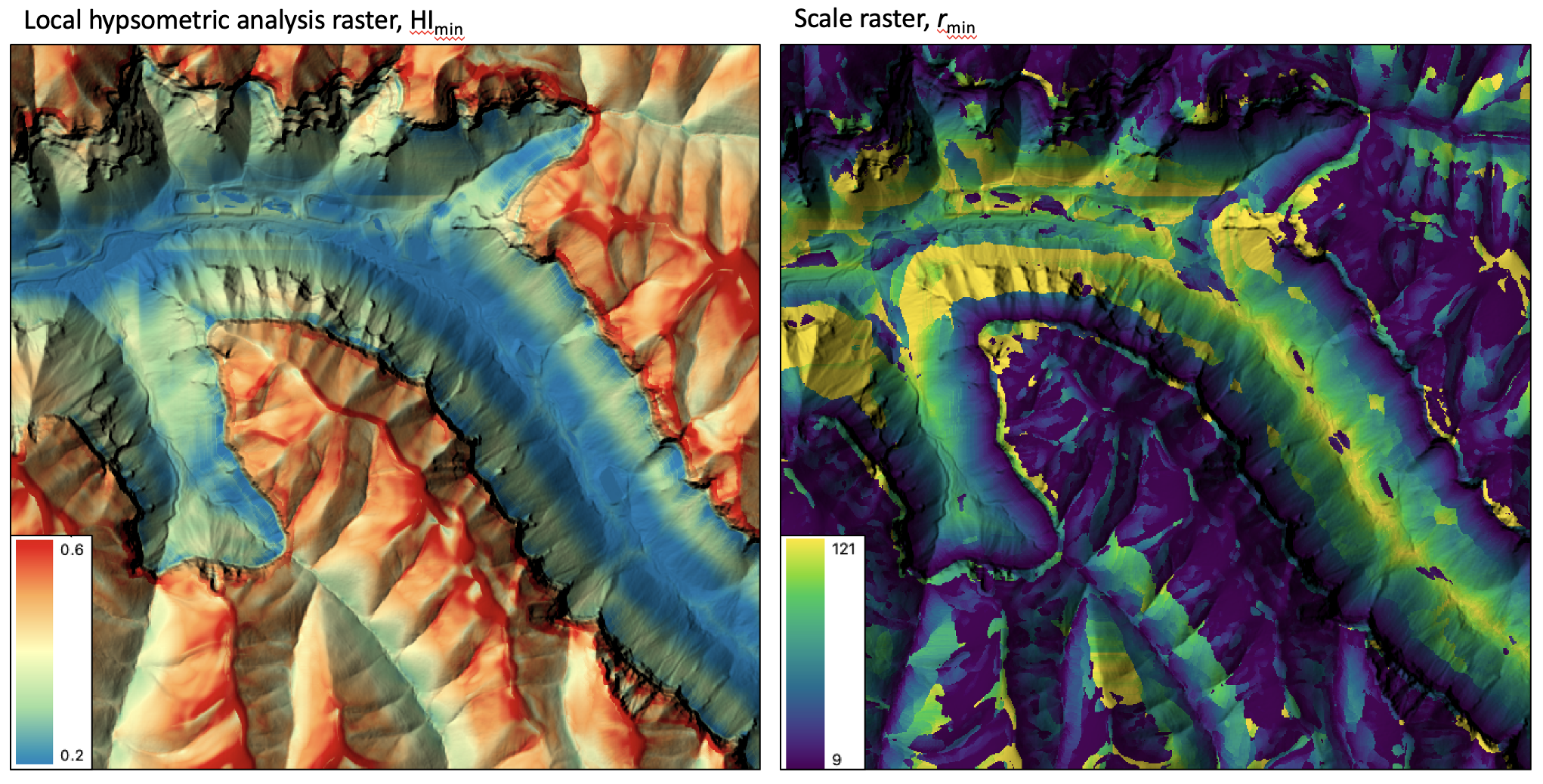
References
Pérez‐Peña, J. V., Azañón, J. M., Booth‐Rea, G., Azor, A., and Delgado, J. (2009). Differentiating geology and tectonics using a spatial autocorrelation technique for the hypsometric integral. Journal of Geophysical Research: Earth Surface, 114(F2).
Pike, R. J., and Wilson, S. E. (1971). Elevation-relief ratio, hypsometric integral, and geomorphic area-altitude analysis. Geological Society of America Bulletin, 82(4), 1079-1084.
See Also
hypsometric_analysis, max_elevation_deviation, multiscale_std_dev_normals
Function Signature
def local_hypsometric_analysis(self, dem: Raster, min_scale: int = 4, step_size: int = 1, num_steps: int = 10, step_nonlinearity: float = 1.0) -> Tuple[Raster, Raster]: ...
logistic_regression
License Information
Use of this function requires a license for Whitebox Workflows for Python Professional (WbW-Pro). Please visit www.whiteboxgeo.com to purchase a license.
Description
This tool performs a logistic regression analysis
using multiple predictor rasters (inputs), or features, and training data (training). Logistic
regression is a type of linear statistical classifier that in its basic form uses a logistic function to
model a binary outcome variable, although the implementation used by this tool can handle multi-class
dependent variables. This tool can be used to model the spatial distribution of class data, such as
land-cover type, soil class, or vegetation type.
The training data take the form of an input vector Shapefile containing a set of points or polygons, for
which the known class information is contained within a field (field) of the attribute table. Each
grid cell defines a stack of feature values (one value for each input raster), which serves as a point within the
multi-dimensional feature space.
The tool splits the training data into two sets, one for training the model and one for testing
the prediction. These test data are used to calculate the classification accuracy stats, as
well as to estimate the variable importance. The test_proportion parameter
is used to set the proportion of the input training data used in model testing. For example, if
test_proportion = 0.2, 20% of the training data will be set aside for testing, and this subset
will be selected randomly. As a result of this random selection of test data, the tool behaves
stochastically, and will result in a different model each time it is run.
Note that the output image parameter (output) is optional. When unspecified, the tool will simply
report the model accuracy statistics and variable importance, allowing the user to experiment with different parameter
settings and input predictor raster combinations to optimize the model before applying it to model the
outcome variable across the whole region defined by image data set.
The user may opt for feature scaling, which can be important when the ranges of the features are different, for
example, if they are measured in different units. Without scaling, features with larger ranges will have
greater influence in computing the distances between points. The tool offers three options for feature-scaling (scaling),
including 'None', 'Normalize', and 'Standardize'. Normalization simply rescales each of the features onto
a 0-1 range. This is a good option for most applications, but it is highly sensitive to outliers because
it is determined by the range of the minimum and maximum values. Standardization
rescales predictors using their means and standard deviations, transforming the data into z-scores. This
is a better option than normalization when you know that the data contain outlier values; however, it does
does assume that the feature data are somewhat normally distributed, or are at least symmetrical in
distribution.
Because the logistic regression calculates distances in feature-space, like many other related algorithms, it suffers from the curse of dimensionality. Distances become less meaningful in high-dimensional space because the vastness of these spaces means that distances between points are less significant (more similar). As such, if the predictor list includes insignificant or highly correlated variables, it is advisable to exclude these features during the model-building phase, or to use a dimension reduction technique such as principal_component_analysis to transform the features into a smaller set of uncorrelated predictors.
See Also
svm_classification, random_forest_classification, knn_classification, principal_component_analysis
Function Signature
def logistic_regression(self, input_rasters: List[Raster], training_data: Vector, class_field_name: str, scaling_method: str = "none", test_proportion: float = 0.2, create_output: bool = False) -> Optional[Raster]: ...
low_points_on_headwater_divides
License Information
Use of this function requires a license for Whitebox Workflows for Python Professional (WbW-Pro). Please visit www.whiteboxgeo.com to purchase a license.
Description
This tool locates low points, or passes, on the drainage divides between subbasins that are situated on headwater divides. A subbasin is the catchment draining to a link in a stream network. A headwater catchment is the portion of a subbasin that drains to the channel head. Only first-order streams contain channel heads and headwater catchments are sometimes referred to as zero-order basins. The lowest points along a zero-order catchment is likely to coincide with mountain passes in alpine environments.
The user must input a depressionless DEM (i.e. a DEM that has been pre-processed to remove all topographic depressions) and a raster stream network. The tool will work best if the raster stream network, generally derived by thresholding a flow-accumulation raster, is processed to remove shorter headwater streams. You can use the remove_short_streams tool remove shorter streams in the input raster. It is recommended to remove streams shorter than 2 or 3 grid cells in length. The algorithm proceeds by first deriving the D8 flow pointer from the input DEM. It then identifies all channel head cells in the input streams raster and the zero-order basins that drain to them. The stream network is then processed to assign a unique identifier to each segment, which is then used to extract subbasins. Lastly, zero-order basin edge cells are identified and the location of lowest grid cells for each pair of neighbouring basins is entered into the output vector file.
See Also
Function Signature
def low_points_on_headwater_divides(self, dem: Raster, streams: Raster) -> Vector: ...
min_dist_classification
License Information
Use of this function requires a license for Whitebox Workflows for Python Professional (WbW-Pro). Please visit www.whiteboxgeo.com to purchase a license.
Description
This tool performs a supervised minimum-distance classification using training site polygons (polys) and
multi-spectral images (inputs). This classification method uses the mean vectors for each class and
calculates the Euclidean distance from each unknown pixel to the class mean vector. Unclassed pixels are
then assigned to the nearest class mean. A threshold distance (threshold), expressed in number of z-scores,
may optionally be used and pixels whose multi-spectral distance is greater than this threshold will not be
assigned a class in the output
image (output). When a threshold distance is unspecified, all pixels will be assigned to a class.
Like all supervised classification methods, this technique relies heavily on proper selection of training data. Training sites are exemplar areas of known and representative land cover type. The algorithm determines the spectral signature of the pixels within each training area, and uses this information to define the mean vector of each class. It is preferable that training sites are based on either field-collected data or fine-resolution reference imagery. In selecting training sites, care should be taken to ensure that they cover the full range of variability within each class. Otherwise the classification accuracy will be impacted. If possible, multiple training sites should be selected for each class. It is also advisable to avoid areas near the edges of land-cover patches, where mixed pixels may impact the purity of training site reflectance values.
After selecting training sites, the reflectance values of each land-cover type can be assessed using the evaluate_training_sites tool. In particular, the distribution of reflectance values should ideally be non-overlapping in at least one band of the multi-spectral data set.
See Also
evaluate_training_sites, parallelepiped_classification
Function Signature
def min_dist_classification(self, input_rasters: List[Raster], training_data: Vector, class_field_name: str, dist_threshold: float = float('inf')) -> Raster: ...
Function Signature
def min_dist_classification(self, input_rasters: List[Raster], training_data: Vector, class_field_name: str, dist_threshold: float = float('inf')) -> Raster: ...
minimal_dispersion_flow_algorithm
License Information
Use of this function requires a license for Whitebox Workflows for Python Professional (WbW-Pro). Please visit www.whiteboxgeo.com to purchase a license.
This function is used to generate flow-direction (pointer) and flow accumulation (catchment area) grids using the
minimal dispersion flow algorithm (MDFA) (Lindsay 2025). MDFA can be run either as a non-dispersive (i.e., single
flow direction) or minimally dispersive (multiple flow direction) flow aglorithm depending on the value of the
path_corrected_direction_preference parameter (p). Dispersive algorithms are sometimes preferred for
some hydrological modelling applications because they overcome the limitations of the main non-dispersive (or
single direction) method, D8, specifically the unnatural appearing extensive straight/parallel flow patterns
and the abundance of artifact source cells (ASCs). An ASC is a cell in a flow-direction (FD) raster that has no
inflowing cells but is not situated at a summit within the digital elevation model. They represent locations
where a flow line has been truncated in the upslope direction, disconnecting the flow line from its starting
peak. Attempts to address the unnatural flow patterns of D8 using alternate non-dispersive flow algorithms (e.g., Rho8) have
resulted in more abundant ASCs. Dispersive flow algorithms can yield more natural appearing flow patterns than
D8 while reducing or eliminating ASCs. However, some researchers have argued that dispersion has little physical
basis in the definition of upslope area and should be minimized in the formulation of these methods. It seems
that a fundamental compromise in flow-path modelling exists between natural-looking flow patterns, the abundance
of ASCs, and the need for dispersion. MDFA restricts dispersion to locations where it is necessary to resolve ASCs
in a non-dispersive path-corrected FD raster.
Flow directions are stored using the same base-2 convention commonly used with FD8, allowing for pointers to multiple neighbors using a single value stored in each grid cell. For example, a cell flowing to its third and fourth neighbors (corresponding to the SE and S cells, if using the convention of ordering cells in a 3x3 starting from the NE and progressing clockwise) has an FD of 23-1 + 24-1 = 12. A summit cell, flowing to all eight neighbors, would have an FD value of 20 + 21 … + 27 = 255.
The FD raster is used as the input for a flow-accumulation operation to create the final MDFA contributing area (CA), or specific contributing area (SCA) grid. For any cell [r, c], the proportion of area (flow) directed towards neighboring cell, i, (Fi) is calculated as:
F_i = p+(1-p)⁄N_out for i = FD_PC
F_i = (1-p)⁄N_out for i != FD_PC
where N_out is the number of outflowing neighbors of cell [r, c], FD_PC is the non-dispersive flow direction determined by the path-correcting algorithm, and p is the proportion of flow (0-1) that is given to FD_PC over and above any other secondary outflowing neighbors. This parameter preserves a preference toward the path-corrected direction in the flow accumulation grid. With p=0.0 (0%) there is no preference for any outflowing cell; with p=1.0 (100%) cells with multiple FDs will direct their flow entirely towards the original path-corrected direction and the algorithm behaves like a non-dispersive method. Therefore, MDFA has the flexibility of being either entirely non-dispersive (p=1.0) or partially dispersive (p<1.0). With p<1.0, it can be said that MDFA is minimally dispersive, since only a small subset of cells needed to eliminate ASCs will be dispersive.
MDFA aims to produce more natural flow patterns than D8, no ASCs, like fully dispersive algorithms (FD8), and substantially less overall dispersion than current dispersion-limiting methods (D-infinity). By limiting dispersion to cells where it is needed to ensure there are no ASCs, MDFA produces FD rasters where every grid cell is connected by a flow path to a downslope outlet cell and upslope to a summit, while most cells have a path-corrected (aspect aligned) single flow direction. MDFA occupies an optimal position in the fundamental flow-path modelling compromise between the needs for realistic flow patterns, no ASCs, and minimal use of dispersion.
The user must spectify the out_type parameter, with values of either "cells", "ca" (total catchment area), or "sca" (specific catchment area). Grid cells possessing the NoData value in the input DEM/pointer raster are assigned the NoData value in the output flow-accumulation image.
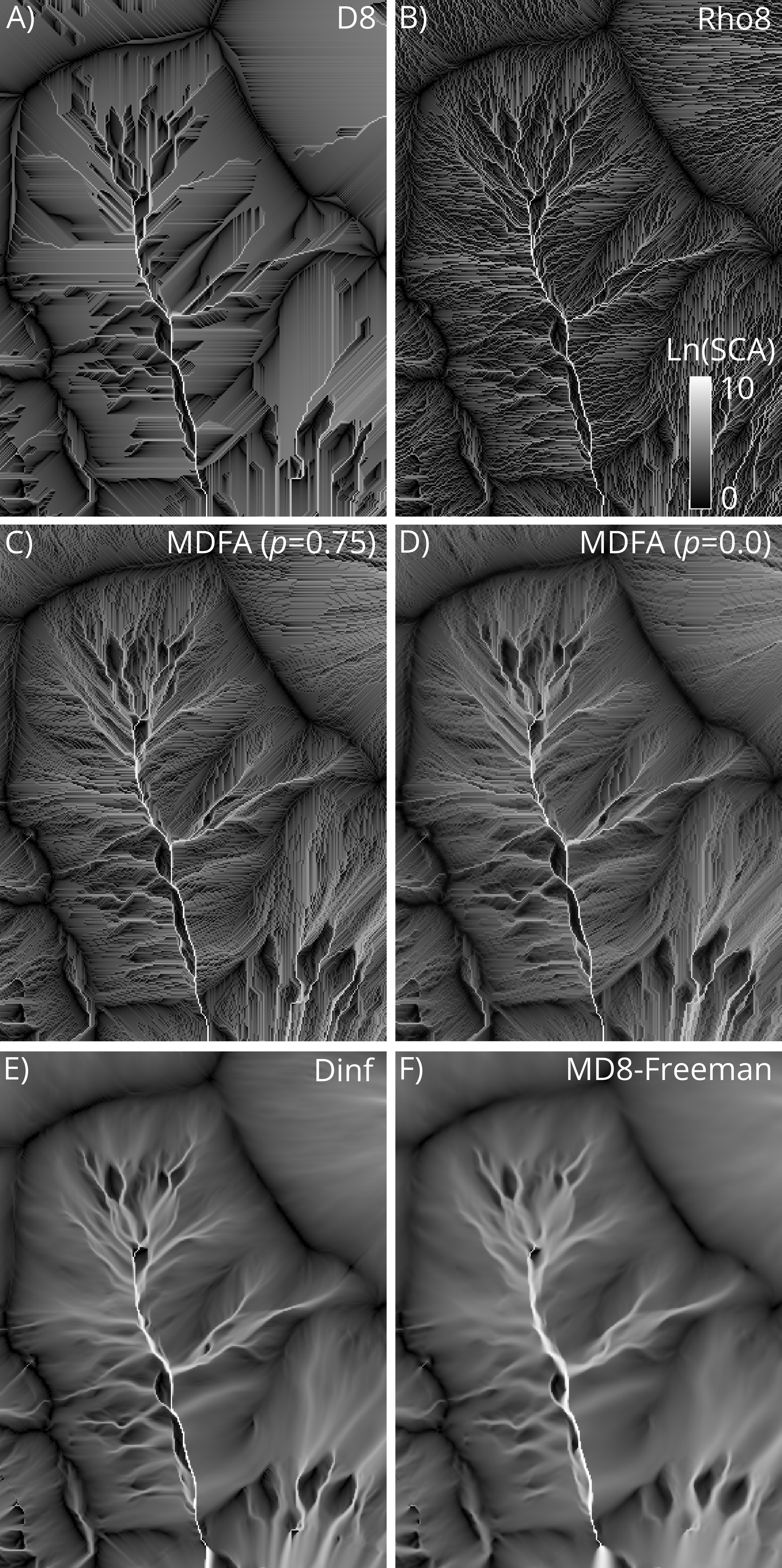
Example Code
from whitebox_workflows import WbEnvironment

wbe = WbEnvironment()

try:
    wbe.verbose = True
    wbe.working_directory = "/path/to/data"

    # Read the input DEM
    dem = wbe.read_rasters('DEM.tif') # Must be depressionless

    flow_dir, flow_accum = wbe.minimal_dispersion_flow_algorithm(dem, out_type='sca', path_corrected_direction_preference=0.5, log_transform=True)
    wbe.write_raster(flow_dir, 'mdfa_flow_direction.tif', compress=True)
    wbe.write_raster(flow_accum, 'mdfa_flow_accumulation.tif', compress=True)

    print('All done!')
except Exception as e:
    print("The error raised is: ", e)
Reference
Lindsay, J.B. 2025. A minimal dispersion flow algorithm. Geomorphometry 2025, Annual Conference of the International Society for Geomorphometry, June 9-13, Perugia, Italy.
See Also:
quinn_flow_accumulation, qin_flow_accumulation, DInfFlowAccumulation, MDInfFlowAccumulation, rho8_pointer, d8_pointer, breach_depressions_least_cost, fill_depressions
Function Signature
def minimal_dispersion_flow_algorithm(self, raster: Raster, out_type: str = "sca", path_corrected_direction_preference: float=0.0, log_transform: bool = False, clip: bool = False, input_is_pointer: bool = False, esri_pntr: bool = False) -> Tuple[Raster, Raster]: ...
modify_lidar
License Information
Use of this function requires a license for Whitebox Workflows for Python Professional (WbW-Pro). Please visit www.whiteboxgeo.com to purchase a license.
Description
The ModifyLidar tool can be used to alter the properties of points within a LiDAR point cloud. The user
provides a statement (statement) containing one or more expressions, separated by semicolons (;).
The expressions are evaluated for each point within the input LiDAR file (input). Expressions assign
altered values to the properties of points in the output file (output), based on any mathematically
defined expression that may include the various properties of individual points (e.g. coordinates, intensity,
return attributes, etc) or some file-level properties (e.g. min/max coordinates). As a basic example, the
following statement:
x = x + 1000.0
could be used to translate the point cloud 1000 x-units (note, the increment operator could be
used as a simpler equivalent, x += 1000.0).
Note that if the user does not specify the optional input LiDAR file, the tool will search for all valid LiDAR (*.las, *.laz, *.zlidar) files contained within the current working directory. This feature can be useful for processing a large number of LiDAR files in batch mode. When this batch mode is applied, the output file names will be the same as the input file names but with a '_modified' suffix added to the end.
Expressions may contain any of the following point-level or file-level variables:
| Variable Name | Description | Type |
|---|---|---|
| Point-level properties | ||
| x | The point x coordinate | float |
| y | The point y coordinate | float |
| z | The point z coordinate | float |
| xy | An x-y coordinate tuple, (x, y) | (float, float) |
| xyz | An x-y-z coordinate tuple, (x, y, z) | (float, float, float) |
| intensity | The point intensity value | int |
| ret | The point return number | int |
| nret | The point number of returns | int |
| is_only | True if the point is an only return (i.e. ret == nret == 1), otherwise false | Boolean |
| is_multiple | True if the point is a multiple return (i.e. nret > 1), otherwise false | Boolean |
| is_early | True if the point is an early return (i.e. ret == 1), otherwise false | Boolean |
| is_intermediate | True if the point is an intermediate return (i.e. ret > 1 && ret < nret), otherwise false | Boolean |
| is_late | True if the point is a late return (i.e. ret == nret), otherwise false | Boolean |
| is_first | True if the point is a first return (i.e. ret == 1 && nret > 1), otherwise false | Boolean |
| is_last | True if the point is a last return (i.e. ret == nret && nret > 1), otherwise false | Boolean |
| class | The class value in numeric form, e.g. 0 = Never classified, 1 = Unclassified, 2 = Ground, etc. | int |
| is_noise | True if the point is classified noise (i.e. class == 7 | |
| is_synthetic | True if the point is synthetic, otherwise false | Boolean |
| is_keypoint | True if the point is a keypoint, otherwise false | Boolean |
| is_withheld | True if the point is withheld, otherwise false | Boolean |
| is_overlap | True if the point is an overlap point, otherwise false | Boolean |
| scan_angle | The point scan angle | int |
| scan_direction | True if the scanner is moving from the left towards the right, otherwise false | Boolean |
| is_flightline_edge | True if the point is situated along the filightline edge, otherwise false | Boolean |
| user_data | The point user data | int |
| point_source_id | The point source ID | int |
| scanner_channel | The point scanner channel | int |
| time | The point GPS time, if it exists, otherwise 0 | float |
| rgb | A red-green-blue tuple (r, g, b) if it exists, otherwise (0,0,0) | (int, int, int) |
| nir | The point near infrared value, if it exists, otherwise 0 | int |
| pt_num | The point number within the input file | int |
| File-level properties (invariant) | ||
| n_pts | The number of points within the file | int |
| min_x | The file minimum x value | float |
| mid_x | The file mid-point x value | float |
| max_x | The file maximum x value | float |
| min_y | The file minimum y value | float |
| mid_y | The file mid-point y value | float |
| max_y | The file maximum y value | float |
| min_z | The file minimum z value | float |
| mid_z | The file mid-point z value | float |
| max_z | The file maximum z value | float |
| x_scale_factor | The file x scale factor | float |
| y_scale_factor | The file y scale factor | float |
| z_scale_factor | The file z scale factor | float |
| x_offset | The file x offset | float |
| y_offset | The file y offset | float |
| z_offset | The file z offset | float |
Most of the point-level properties above are modifiable, however some are not. The complete list of modifiable point attributes include, x, y, z, xy, xyz, intensity, ret, nret, class, user_data, point_source_id, scanner_channel, scan_angle, time, rgb, nir, is_synthetic, is_keypoint, is_withheld, and is_overlap. The immutable properties include is_only, is_multiple, is_early, is_intermediate, is_late, is_first, is_last, is_noise, and pt_num. Of the file-level properties, the modifiable properties include the x_scale_factor, y_scale_factor, z_scale_factor, x_offset, y_offset, and z_offset.
In addition to the point properties defined above, if the user applies the lidar_eigenvalue_features
tool on the input LiDAR file, the modify_lidar tool will automatically read in the additional *.eigen
file, which include the eigenvalue-based point neighbourhood measures, such as lambda1, lambda2, lambda3,
linearity, planarity, sphericity, omnivariance, eigentropy, slope, and residual. See the
lidar_eigenvalue_features documentation for details on each of these metrics describing the structure
and distribution of points within the neighbourhood surrounding each point in the LiDAR file.
Expressions may use any of the standard mathematical operators, +, -, *, /, % (modulo), ^ (exponentiation),
comparison operators, <, >, <=, >=, == (equality), != (inequality), and logical operators, && (Boolean AND),
|| (Boolean OR). Expressions must evaluate to an assignment operation, where the variable that is assigned
to must be a modifiable point-level property (see table above). That is, expressions should take the form
pt_variable = .... Other assignment operators are also possible (at least for numeric non-tuple properties),
such as the increment (=+) operator (e.g. x += 1000.0) and the decrement (-=) operator (e.g. y -= 1000.0).
Expressions may use a number of built-in mathematical functions, including:
| Function Name | Description | Example |
|---|---|---|
| if | Performs an if(CONDITION, TRUE, FALSE) operation, return either the value of TRUE or FALSE depending on CONDITION | ret = if(ret==0, 1, ret) |
| abs | Returns the absolute value of the argument | value = abs(x - mid_x) |
| min | Returns the minimum of the arguments | value = min(x, y, z) |
| max | Returns the maximum of the arguments | value = max(x, y, z) |
| floor | Returns the largest integer less than or equal to a number | x = floor(x) |
| round | Returns the nearest integer to a number. Rounds half-way cases away from 0.0 | x = round(x) |
| ceil | Returns the smallest integer greater than or equal to a number | x = ceil(x) |
| clamp | Forces a value to fall within a specified range, defined by a minimum and maximum | z = clamp(min_z+10.0, z, max_z-20.0) |
| int | Returns the integer equivalent of a number | intensity = int(z) |
| float | Returns the float equivalent of a number | z = float(intensity) |
| to_radians | Converts a number in degrees to radians | val = to_radians(scan_angle) |
| to_degrees | Converts a number in radians to degrees | scan_angle = int(to_degrees(val)) |
| dist | Returns the distance between two points defined by two n-length tuples | d = dist(xy, (mid_x, mid_y)) or d = dist(xyz, (mid_x, mid_y, mid_z)) |
| rotate_pt | Rotates an x-y point by a certain angle, in degrees | xy = rotate_pt(xy, 45.0) or orig_pt = (1000.0, 1000.0); xy = rotate_pt(xy, 45.0, orig_pt) |
| math::ln | Returns the natural logarithm of the number | z = math::ln(z) |
| math::log | Returns the logarithm of the number with respect to an arbitrary base | z = math::log(z, 10) |
| math::log2 | Returns the base 2 logarithm of the number | z = math::log2(z) |
| math::log10 | Returns the base 10 logarithm of the number | z = math::log10(z) |
| math::exp | Returns e^(number), (the exponential function) | z = math::exp(z) |
| math::pow | Raises a number to the power of the other number | z = math::pow(z, 2.0) |
| math::sqrt | Returns the square root of a number. Returns NaN for a negative number | z = math::sqrt(z, 2.0) |
| math::cos | Computes the cosine of a number (in radians) | z = math::cos(to_radians(z)) |
| math::sin | Computes the sine of a number (in radians) | z = math::sin(to_radians(z)) |
| math::tan | Computes the tangent of a number (in radians) | z = math::tan(to_radians(z)) |
| math::acos | Computes the arccosine of a number. The return value is in radians in the range [0, pi] or NaN if the number is outside the range [-1, 1] | z = math::acos(z) |
| math::asin | Computes the arcsine of a number. The return value is in radians in the range [0, pi] or NaN if the number is outside the range [-1, 1] | z = math::asin(z) |
| math::atan | Computes the arctangent of a number. The return value is in radians in the range [0, pi] or NaN if the number is outside the range [-1, 1] | z = math::atan(z) |
| rand | Returns a random value between 0 and 1, with an optional seed value | rgb = (int(255.0 * rand()), int(255.0 * rand()), int(255.0 * rand())) |
| helmert_transformation | Performs a Helmert transformation on a point using a 7-parameter transform | xyz = helmert_transformation(xyz, −446.448, 125.157, −542.06, 20.4894, −0.1502, −0.247, −0.8421 ) |
The hyperbolic trigonometric functions are also available for use in expression building, as is math::atan2
and the mathematical constants pi and e.
You may use if operations within statements to implement a conditional modification of point properties.
For example, the following expression demonstrates how you could modify a point's RGB colour based on its
classification, assign ground points (class 2) in the output file a green colour:
rgb = if(class==2, (0,255,0), rgb)
To colour all points within 50 m of the tile mid-point red and all other points blue:
rgb = if(dist(xy, (mid_x, mid_y))<50.0, (255,0,0), (0,0,255))
if operations may also be nested to create more complex compound conditional point modification. For example,
in the following statement, we assign first-return points red (255,0,0) and last-return points green (0,255,0)
colours and white (255,255,255) to all other points (intermediate-returns and only-returns):
rgb = if(is_first, (255,0,0), if(is_last, (0,255,0), (255,255,255)))
Here we use an if expression to re-classify points above an elevation of 1000.0 as high noise (class 18):
class = if(z>1000.0, 18, class)
Expressions may be strung together within statements using semicolons (;), with each expression being evaluated individually. When this is the case, at least one of the expressions must assign a value to one of the variant point properties (see table above). The following statement demonstrates multi-expression statements, in this case to swap the x and y coordinates in a LiDAR file:
new_var = x; x = y; y = new_var
The rand function, used with the seeding option, can be useful when assigning colours to points based on
common point properties. For example, to assign a point a random RGB colour based on its point_source_id
(Note, for many point clouds, this operation will assign each flightline a unique colour; if flightline
information is not stored in the file's point_source_id attribute, one could use the recover_flightline_info
tool to calculate this data.):
rgb=(int(255 * rand(point_source_id)), int(255 * rand(point_source_id+1)), int(255 * rand(point_source_id+2)))
This expression-based approach to modifying point properties provides a great deal of flexibility and power to the processing of LiDAR point cloud data sets.
See Also
filter_lidar, sort_lidar, lidar_eigenvalue_features
Function Signature
def modify_lidar(self, statement: str, input_lidar: Optional[Lidar]) -> Optional[Lidar]: ...
multiscale_curvatures
License Information
Use of this function requires a license for Whitebox Workflows for Python Professional (WbW-Pro). Please visit www.whiteboxgeo.com to purchase a license.
Description
This tool calculates several multiscale curvatures and curvature-based indices from an input DEM (dem). There
are 18 curvature types (curv_type) available, including: accumulation curvature, curvedness, difference curvature,
Gaussian curvature, generating function, horizontal excess curvature, maximal curvature, mean curvature, minimal
curvature, plan curvature, profile curvature, ring curvature, rotor, shape index, tangential curvature, total
curvature, unsphericity, and vertical excess curvature. Each of these curvatures can be measured in non-multiscale
fashion using the corresponding tools available in either the WhiteboxTools open-core or the Whitebox extension.
Like many of the multi-scale land-surface parameter tools available in Whitebox, this tool can be run in two different modes: it can either be used to measure curvature at a single specific scale or to generate a curvature scale mosaic. To understand the difference between these two modes, we must first understand how curvatures are measured and how the non-multiscale curvature tools (e.g. profile_curvature) work. Curvatures are generally measured by fitting a mathematically defined surface to the elevation values within the local neighbourhood surrounding each grid cell in a DEM. The Whitebox curvature tools use the algorithms described Florinsky (2016), which use the 25 elevations within a 5 x 5 local neighbouhood for projected DEMs, and the nine elevations within a 3 x 3 neighbourhood for DEMs in geographic coordinate systems. This is what determines the scale at which these land-surface parameters are calculated. Because they are calculated using small local neighbourhoods (kernels), then these algorithms are heavily impacted by micro-topographic roughness and DEM noise. For example, in a fine-resolution DEM containing a great deal of micro-topographic roughness, the measured curvature value will be dominated by topographic variation at the scale of the roughness rather than the hillslopes on which that roughness is superimposed. This mis-matched scaling can be a problem in many applications, e.g. in landform classification and slope failure modelling applications.
Using the multiscale_curvatures tool, the user can specify a certain desired scale, larger than that defined by the grid resolution
and kernel size, over which a curvature should be characterized. The tool will then use a fast
Gaussian scale-space method to remove the topographic variation in the
DEM at scales less than the desired scale, and will then characterize the curvature using the usual method based on
this scaled DEM. To measure curvature at a single non-local scale, the user must specify a minimum search neighbourhood
radius in grid cells (min_scale) greater than 0.0. Note that a minimum search neighbourhood of 0.0 will replicate the non-multiscale
equivalent curvature tool and any min_scale value > 0.0 will apply the Gassian scale space method to eliminate
topographic variation less than the scale of the minimum search neighbourhood. The base step size (step), number of steps (num_steps), and step
nonlinearity (step_nonlinearity) parameters should all be left to their default values of 1 in this case. The
output curvature raster will be written to the output magnitude file (out_mag). The following animation shows
several multiscale curvature rasters (tangential curvature) measured from a DEM across a range of spatial scales.
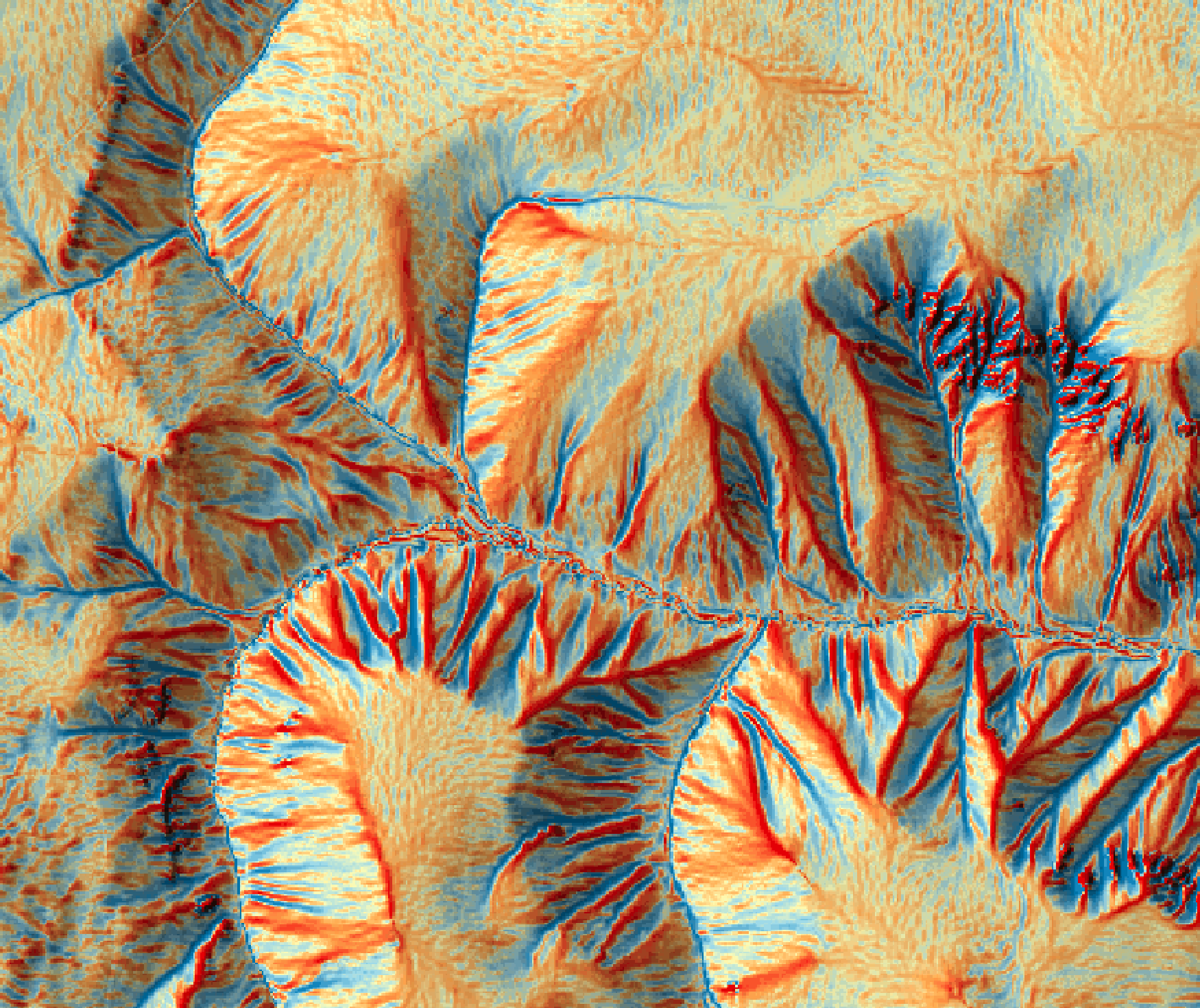
Alternatively, one can use this tool to create a curvature scale mosaic. In this case, the user specifies a range of
spatial scales (i.e., a scale space) over which to measure curvature. The curvature scale-space is densely sampled
and each grid cell is assigned the maximum absolute curvature value (for the specified curvature type) across the
scale space. In this scale-mosaic mode, the user must also specify the output scale file name (out_scale), which
is an output raster that, for each grid cell, specifies the scale at which the maximum absolute curvature was identified.
The following is an example of a scale mosaic of unsphericity for an area in Pole Canyon, Utah (min_scale=1.0,
step=1, num_steps=50, step_nonlinearity=1.0).
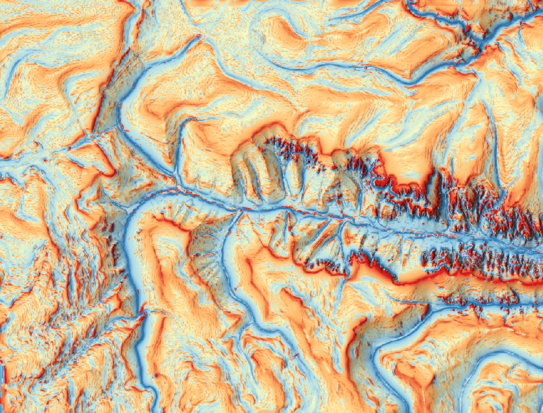
Scale mosaics are useful when modelling spatial distributions of land-surface parameters, like curvatures, in complex and heterogeneous landscapes that contain an abundance of topographic variation (micro-topography, landforms, etc.) at widely varying spatial scales, often associated with different geomorphic processes. Notice how in the image above, relatively strong curvature values are being characterized for both the landforms associated with the smaller-scale mass-movement processes as well as the broader-scale fluvial erosion (i.e. valley incision and hillslopes). It would be difficult, or impossible, to achieve this effect using a single, uniform scale. Each location in a land-surface parameter scale mosaic represents the parameter measured at a characteristic scale, given the unique topography of the site and surroundings.
The properties of the sampled scale space are
determined using the min_scale, step, num_steps (greater than 1), and step_nonlinearity parameters.
Experience with multiscale curvature scales spaces has shown that they are more highly variable at shorter spatial
scales and change more gradually at broader scales. Therefore, a nonlinear scale sampling interval is used by this
tool to ensure that the scale sampling density is higher for short scale ranges and coarser at longer tested scales,
such that:
ri = rL + [step × (i - rL)]p
Where ri is the filter radius for step i and p is the nonlinear scaling factor (step_nonlinearity)
and a step size (step) of step.
In scale-mosaic mode, the user must also decide whether or not to standardize the curvature values (standardize).
When this parameter is used, the algorithm will convert each curvature raster associated with each sampled region
of scale-space to z-scores (i.e. differenced from the raster-wide mean and divided by the raster-wide standard
deviation). It it usually the case that curvature values measured at broader spatial scales will on the whole
become less strongly valued. Because the scale mosaic algorithm used in this tool assigns each grid cell the
maximum absolute curvature observed within sampled scale-space, this implies that the curvature values associated
with more local-scale ranges are more likely to be selected for the final scale-mosaic raster. By standardizing
each scaled curvature raster, there is greater opportunity for the final scale-mosaic to represent broader
scale topographic variation. Whether or not this is appropriate will depend on the application. However, it
is important to stress that the sampled scale-space need not span the full range of possible scales, from the finest
scale determined by the grid resolution up to the broadest scale possible, determined by the spatial extent of
the input DEM. Often, a better approach is to use this tool to create multiple scale mosaics spanning this range,
thereby capturing variation within broadly defined scale ranges. For example, one could create a local-scale, meso-scale,
and broad-scale curvature scale mosaics, each of which would capture topographic variation and landforms that are
present in the landscape and reflective of processing operating at vastly different spatial scales. When this approach
is used, it may not be necessary to standardize each scaled curvature raster, since the gradual decline in
curvature values as scales increase is less pronounced within each of these broad scale ranges than across the
entirety of possible scale-space. Again, however, this will depend on the application and on the characteristics of
the landscape at study.
Raw curvedness values are often challenging to visualize given their range and magnitude,
and as such the user may opt to log-transform the output raster (log). Transforming the values
applies the equation by Shary et al. (2002):
Θ' = sign(Θ) ln(1 + 10n|Θ|)
where Θ is the parameter value and n is dependent on the grid cell size.
References
Florinsky, I. (2016). Digital terrain analysis in soil science and geology. Academic Press.
See Also
gaussian_scale_space, accumulation_curvature, curvedness, difference_curvature, gaussian_curvature,
generating_function, horizontal_excess_curvature, maximal_curvature, mean_curvature, minimal_curvature,
plan_curvature, profile_curvature, ring_curvature, rotor, shape_index, tangential_curvature,
total_curvature, unsphericity, vertical_excess_curvature
Function Signature
def multiscale_curvatures(self, dem: Raster, curv_type: str = 'profile', min_scale: int = 4, step_size: int = 1, num_steps: int = 10, step_nonlinearity: float = 1.0, log_transform: bool = True, standardize: bool = False) -> Tuple[Raster, Raster]: ...
nibble
Use of this function requires a license for Whitebox Workflows for Python Professional (WbW-Pro). Please visit www.whiteboxgeo.com to purchase a license.
The nibble function assigns areas within an input class map raster that are coincident with a mask the value of their nearest neighbour. Nibble is typically used to replace erroneous sections in a class map. Cells in the mask raster that are either NoData or zero values will be replaced in the input image with their nearest non-masked value. All input raster values in non-mask areas will be unmodified.
There are two input parameters that are related to how NoData cells in the input raster are handled during the nibble operation. The use_nodata Boolean determines whether or not input NoData cells, not contained within masked areas, are treated as ordinary values during the nibble. It is False by default, meaning that NoData cells in the input raster do not extend into nibbled areas. When the nibble_nodata parameter is True, any NoData cells in the input raster that are within the masked area are also NoData in the output raster; when nibble_nodata is False these cells will be nibbled.
See Also:
Function Signature
def nibble(self, input_raster: Raster, mask: Raster, use_nodata: bool = False, nibble_nodata: bool = True) -> Raster:
openness
License Information
Use of this function requires a license for Whitebox Workflows for Python Professional (WbW-Pro). Please visit www.whiteboxgeo.com to purchase a license.
Description
This tool calculates the Yokoyama et al. (2002) topographic openness index from an input DEM (input).
Openness has two viewer perspectives, which correspond with positive and negative openness outputs (pos_output
and neg_output). Positive values, expressing openness above the surface, are high for convex forms,
whereas negative values describe this attribute below the surface and are high for concave forms. Openness
is an angular value that is an average of the horizon angle in the eight cardinal directions to a maximum
search distance (dist), measured in grid cells. Openness rasters are best visualized using a greyscale palette.
Positive Openness:
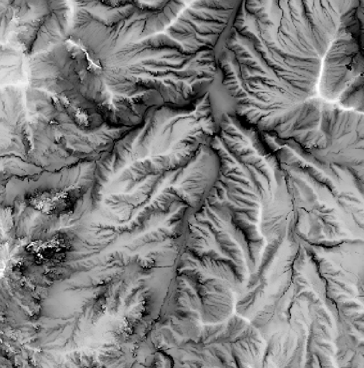
Negative Openness:
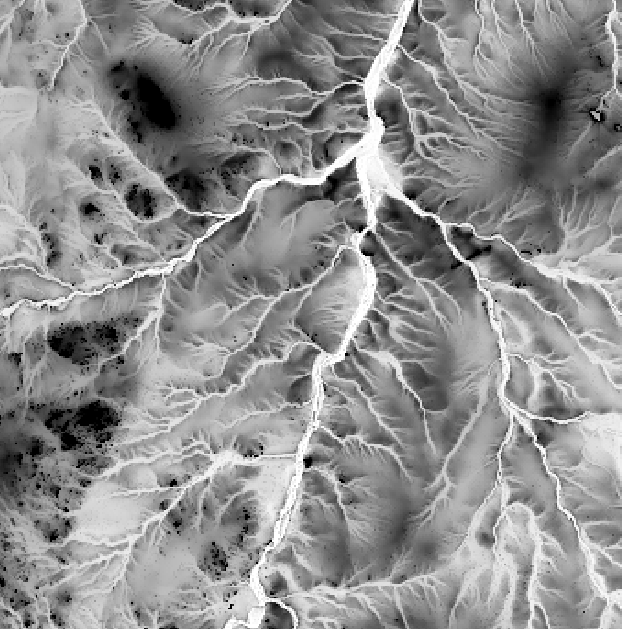
References
Yokoyama, R., Shirasawa, M., & Pike, R. J. (2002). Visualizing topography by openness: a new application of image processing to digital elevation models. Photogrammetric engineering and remote sensing, 68(3), 257-266.
See Also
viewshed, horizon_angle, time_in_daylight, hillshade
Function Signature
def openness(self, dem: Raster, dist: int = 20) -> Tuple[Raster, Raster]: ...
parallelepiped_classification
License Information
Use of this function requires a license for Whitebox Workflows for Python Professional (WbW-Pro). Please visit www.whiteboxgeo.com to purchase a license.
Description
This tool performs a supervised parallelepiped classification
using training site polygons (polys) and multi-spectral images (inputs). This classification method
uses the minimum and maximum reflectance values for each class within the training data to characterize a set
of parallelepipeds, i.e. multi-dimensional geometric shapes.
The algorithm then assigns each unknown pixel in the image data set to the first class for which the pixel's
spectral vector is contained within the corresponding class parallelepiped. Pixels with spectral vectors that
are not contained within any class parallelepiped will not be assigned a class in the output image.
Like all supervised classification methods, this technique relies heavily on proper selection of training data. Training sites are exemplar areas of known and representative land cover type. The algorithm determines the spectral signature of the pixels within each training area, and uses this information to define the mean vector of each class. It is preferable that training sites are based on either field-collected data or fine-resolution reference imagery. In selecting training sites, care should be taken to ensure that they cover the full range of variability within each class. Otherwise the classification accuracy will be impacted. If possible, multiple training sites should be selected for each class. It is also advisable to avoid areas near the edges of land-cover patches, where mixed pixels may impact the purity of training site reflectance values.
After selecting training sites, the reflectance values of each land-cover type can be assessed using the evaluate_training_sites tool. In particular, the distribution of reflectance values should ideally be non-overlapping in at least one band of the multi-spectral data set.
See Also
evaluate_training_sites, min_dist_classification
Function Signature
def parallelepiped_classification(self, input_rasters: List[Raster], training_data: Vector, class_field_name: str) -> Raster: ...
phi_coefficient
License Information
Use of this function requires a license for Whitebox Workflows for Python Professional (WbW-Pro). Please visit www.whiteboxgeo.com to purchase a license.
Description
This tool performs a binary classification accuracy assessment, using the Phi coefficient.
The Phi coefficient is a measure of association for two binary variables. Introduced by Karl Pearson, this measure is
similar to the Pearson correlation coefficient in its interpretation and is related to the chi-squared statistic
for a 2×2 contingency table. The user must specify the names of two input images (input1 and input2), containing
categorical data.
Function Signature
def phi_coefficient(self, raster1: Raster, raster2: Raster, output_html_file: str) -> None: ...
piecewise_contrast_stretch
License Information
Use of this function requires a license for Whitebox Workflows for Python Professional (WbW-Pro). Please visit www.whiteboxgeo.com to purchase a license.
Description
This tool can be used to perform a piecewise contrast stretch on an input image (input). The input image
can be either a single-band image or a colour composite, in which case the contrast stretch will be
performed on the intensity values of the hue-saturation-intensity (HSI) transform of the colour image.
The user must also specify the name of the output image (output) and the break-points that define the
piecewise function used to transfer brightness values from the input to the output image. The break-point
values are specified as a string parameter (function), with each break-point taking the form of
(input value, output proportion); (input value, output proportion); (input value, output proportion), etc.
Piecewise functions can have as many break-points as desired, and each break-point should be separated by
a semicolon (;). The input values are specifies as brightness values in the same units as the input image
(unless it is an input colour composite, in which case the intensity values range from 0 to 1). The output
function must be specified as a proportion (from 0 to 1) of the output value range, which is specified by
the number of output greytones (greytones). The greytones parameter is ignored if the input image
is a colour composite. Note that there is no need to specify the initial break-point to the piecewise
function, as (input min value; 0.0) will be inserted automatically. Similarly, an upper bound of the piecewise
function of (input max value; 1.0) will also be inserted automatically.
Generally you want to set breakpoints by examining the image histogram. Typically it is desirable to map large unpopulated ranges of input brightness values in the input image onto relatively narrow ranges of the output brightness values (i.e. a shallow sloped segment of the piecewise function), and areas of the histogram that are well populated with pixels in the input image with a larger range of brightness values in the output image (i.e. a steeper slope segment). This will have the effect of reducing the number of tones used to display the under-populated tails of the distribution and spreading out the well-populated regions of the histogram, thereby improving the overall contrast and the visual interpretability of the output image. The flexibility of the piecewise contrast stretch can often provide a very suitable means of significantly improving image quality.
See Also
raster_histogram, gaussian_contrast_stretch, min_max_contrast_stretch, standard_deviation_contrast_stretch
Function Signature
def piecewise_contrast_stretch(self, raster: Raster, transformation_statement: str, num_greytones: float = 1024.0) -> Raster: ...
prune_vector_streams
License Information
Use of this function requires a license for Whitebox Workflows for Python Professional (WbW-Pro). Please visit www.whiteboxgeo.com to purchase a license.
Description
This tool can be used to prune the smallest branches of a vector stream network based on a threshold in link magnitude.
The function automatically calculates the Shreve magnitude of each link in the input streams vector. This operation
requires an input digital elevation model (DEM). The function is also capable of calculating the link magnitude from
stream networks that have some minor topological errors (e.g., line overshoots or undershoots). This requires the
input of a snap_distance parameter (default = 0.0).
See Also
vector_stream_network_analysis, repair_stream_vector_topology
Function Signature
def prune_vector_streams(self, streams: Vector, dem: Raster, threshold: float, snap_distance: float = 0.001) -> Vector: ...
random_forest_classification_fit
License Information
Use of this function requires a license for Whitebox Workflows for Python Professional (WbW-Pro). Please visit www.whiteboxgeo.com to purchase a license.
Description
This tool performs a supervised random forest (RF) classification
using multiple predictor rasters (inputs), or features, and training data (training). It can be used to model
the spatial distribution of class data, such as land-cover type, soil class, or vegetation type.
The training data take the form of an input vector Shapefile containing a set of points or polygons, for
which the known class information is contained within a field (class_field_name) of the attribute table. Each
grid cell defines a stack of feature values (one value for each input raster), which serves as a point
within the multi-dimensional feature space. Random forest is an ensemble learning method that works by
creating a large number (n_trees) of decision trees and using a majority vote to determine estimated
class values. Individual trees are created using a random sub-set of predictors. This ensemble approach
overcomes the tendency of individual decision trees to overfit the training data. As such, the RF method
is a widely and successfully applied machine-learning method in many domains.
Note that this function is part of a set of two tools, including random_forest_classification_fit and random_forest_classification_prdict. The random_forest_classificaiton_fit tool should be used first to create the RF model and the random_forest_classification_predict can then be used to apply that model for prediction. The output of the fit tool is a byte array that is a binary representation of the RF model. This model can then be used as the input to the predict tool, along with a list of input raster predictors, which must be in the same order as those used in the fit tool. The output of the predict tool is a classified raster. The reason that the RF workflow is split in this way is that often it is the case that you need to experiment with various input predictor sets and parameter values to create an adequate model. There is no need to generate an output classified raster during this experimentation stage, and because prediction can often be the slowest part of the RF modelling process, it is generally only performed after the final model has been identified. The binary representation of the RF-based model can be serialized (i.e., saved to a file) and then later read back into memory to serve as the input for the prediction step of the workflow (see code example below).
Also note that this tool is for RF-based classification. There is a similar set of fit and *predict tools available for performing RF-based regression, including random_forest_regression_fit and random_forest_regression_predict. These tools are more appropriately applied to the modelling of continuous data, rather than categorical data.
The user must specify the splitting criteria (split_criterion) used in training the decision trees.
Options for this parameter include 'Gini', 'Entropy', and 'ClassificationError'. The model can also
be adjusted based on each of the number of trees (n_trees), the minimum number of samples required to
be at a leaf node (min_samples_leaf), and the minimum number of samples required to split an internal
node (min_samples_split) parameters.
The tool splits the training data into two sets, one for training the classifier and one for testing
the model. These test data are used to calculate the overall accuracy and Cohen's kappa
index of agreement, as well as to estimate the variable importance. The test_proportion parameter
is used to set the proportion of the input training data used in model testing. For example, if
test_proportion = 0.2, 20% of the training data will be set aside for testing, and this subset
will be selected randomly. As a result of this random selection of test data, and the random selection of
features used in decision tree creation, the tool is inherently stochastic, and will result in a
different model each time it is run.
Like all supervised classification methods, this technique relies heavily on proper selection of training data. Training sites are exemplar areas/points of known and representative class value (e.g. land cover type). The algorithm determines the feature signatures of the pixels within each training area. In selecting training sites, care should be taken to ensure that they cover the full range of variability within each class. Otherwise the classification accuracy will be impacted. If possible, multiple training sites should be selected for each class. It is also advisable to avoid areas near the edges of class objects (e.g. land-cover patches), where mixed pixels may impact the purity of training site values.
After selecting training sites, the feature value distributions of each class type can be assessed using the evaluate_training_sites tool. In particular, the distribution of class values should ideally be non-overlapping in at least one feature dimension.
RF, like decision trees, does not require feature scaling. That is, unlike the k-NN algorithm and other methods that are based on the calculation of distances in multi-dimensional space, there is no need to rescale the predictors onto a common scale prior to RF analysis. Because individual trees do not use the full set of predictors, RF is also more robust against the curse of dimensionality than many other machine learning methods. Nonetheless, there is still debate about whether or not it is advisable to use a large number of predictors with RF analysis and it may be better to exclude predictors that are highly correlated with others, or that do not contribute significantly to the model during the model-building phase. A dimension reduction technique such as principal_component_analysis can be used to transform the features into a smaller set of uncorrelated predictors.
Example Code
import os
from whitebox_workflows import WbEnvironment

license_id = 'floating-license-id'
wbe = WbEnvironment(license_id)

try:
    wbe.verbose = True
    wbe.working_directory = "/path/to/data"

    # Read the input raster files into memory
    images = wbe.read_rasters(
        'LC09_L1TP_018030_20220614_20220615_02_T1_B2.TIF',
        'LC09_L1TP_018030_20220614_20220615_02_T1_B3.TIF',
        'LC09_L1TP_018030_20220614_20220615_02_T1_B4.TIF',
        'LC09_L1TP_018030_20220614_20220615_02_T1_B5.TIF'
    )

    # Read the input training polygons into memory
    training_data = wbe.read_vector('training_data.shp')

    # Train the model
    model = wbe.random_forest_classification_fit(
        images,
        training_data,
        class_field_name = 'CLASS',
        split_criterion = "Gini",
        n_trees = 50,
        min_samples_leaf = 1,
        min_samples_split = 2,
        test_proportion = 0.2
    )

    ### Example of how to serialize the model, i.e., save the model, which is just binary data
    print('Saving the model to file...')
    file_path = os.path.join(wbe.working_directory, "rf_model.bin")
    with open(file_path, "wb") as file:
        file.write(bytearray(model))

    ### Example of how to deserialize the model, i.e. read the model
    model = []
    with open(file_path, mode='rb') as file:
        model = list(file.read())

    # Use the model to predict
    rf_class_image = wbe.random_forest_classification_predict(images, model)

    wbe.write_raster(rf_class_image, 'rf_classification.tif', compress=True)

    print('All done!')
except Exception as e:
    print("The error raised is: ", e)
finally:
    wbe.check_in_license(license_id)
See Also
random_forest_classification_predict, random_forest_regression_fit, random_forest_regression_predict, knn_classification, svm_classification, parallelepiped_classification, evaluate_training_sites
Function Signature
def random_forest_classification_fit(self, input_rasters: List[Raster], training_data: Vector, class_field_name: str, split_criterion: str = "gini", n_trees: int = 500, min_samples_leaf: int = 1, min_samples_split: int = 2, test_proportion: float = 0.2) -> List[int]: ...
random_forest_classification_predict
Note this tool is part of a WhiteboxTools extension product. Please visit Whitebox Geospatial Inc. for information about purchasing a license activation key (https://www.whiteboxgeo.com/extension-pricing/).
This tool applies a pre-built random forest (RF) classification
model trained using multiple predictor rasters (input_rasters), or features, and training data to predict
a spatial distribution. This function is part of a set of two tools, including
random_forest_classification_fit
and random_forest_classification_prdict. The
random_forest_classification_fit tool should be used first to create the RF model and the random_forest_classification_predict
can then be used to apply that model for prediction. The output of the fit tool is a byte array that is a
binary representation of the RF model. This model can then be used as the input to the predict tool, along with
a list of input raster predictors, which must be in the same order as those used in the fit tool (see below). The
output of the predict tool is a classified raster. The reason that the RF workflow is split in this way is
that often it is the case that you need to experiment with various input predictor sets and parameter values
to create an adequate model. There is no need to generate an output classified raster during this experimentation
stage, and because prediction can often be the slowest part of the RF modelling process, it is generally only
performed after the final model has been identified. The binary representation of the RF-based model can be
serialized (i.e., saved to a file) and then later read back into memory to serve as the input for the prediction
step of the workflow (see code example below).
Note: it is very important that the order of feature rasters is the same for both fitting the model and using the model for prediction. It is possible to use a model fitted to one data set to make preditions for another data set, however, the set of feature reasters specified to the prediction tool must be input in the same sequence used for building the model. For example, one may train a RF classifer on one set of multi-spectral satellite imagery and then apply that model to classify a different imagery scene, but the image band sequence must be the same for the Fit/Predict tools otherwise inaccurate predictions will result.
Example Code
import os
from whitebox_workflows import WbEnvironment

license_id = 'floating-license-id'
wbe = WbEnvironment(license_id)

try:
    wbe.verbose = True
    wbe.working_directory = "/path/to/data"

    # Read the input raster files into memory
    images = wbe.read_rasters(
        'LC09_L1TP_018030_20220614_20220615_02_T1_B2.TIF',
        'LC09_L1TP_018030_20220614_20220615_02_T1_B3.TIF',
        'LC09_L1TP_018030_20220614_20220615_02_T1_B4.TIF',
        'LC09_L1TP_018030_20220614_20220615_02_T1_B5.TIF'
    )

    # Read the input training polygons into memory
    training_data = wbe.read_vector('training_data.shp')

    # Train the model
    model = wbe.random_forest_classification_fit(
        images,
        training_data,
        class_field_name = 'CLASS',
        split_criterion = "Gini",
        n_trees = 50,
        min_samples_leaf = 1,
        min_samples_split = 2,
        test_proportion = 0.2
    )

    ### Example of how to serialize the model, i.e., save the model, which is just binary data
    print('Saving the model to file...')
    file_path = os.path.join(wbe.working_directory, "rf_model.bin")
    with open(file_path, "wb") as file:
        file.write(bytearray(model))

    ### Example of how to deserialize the model, i.e. read the model
    model = []
    with open(file_path, mode='rb') as file:
        model = list(file.read())

    # Use the model to predict
    rf_class_image = wbe.random_forest_classification_predict(images, model)

    wbe.write_raster(rf_class_image, 'rf_classification.tif', compress=True)

    print('All done!')
except Exception as e:
    print("The error raised is: ", e)
finally:
    wbe.check_in_license(license_id)
See Also
random_forest_classification_fit, random_forest_regression_fit, random_forest_regression_predict, knn_classification, svm_classification, parallelepiped_classification, evaluate_training_sites
Function Signature
def random_forest_classification_predict(self, input_rasters: List[Raster], model_bytes: List[int]) -> Raster: ...
random_forest_regression_fit
License Information
Use of this function requires a license for Whitebox Workflows for Python Professional (WbW-Pro). Please visit www.whiteboxgeo.com to purchase a license.
Description
This function performs a supervised random forest (RF) regression analysis
using multiple predictor rasters (input_rasters), or features, and training data (training_data).
The training data take the form of an input vector Shapefile containing a set of points, for
which the known outcome information is contained within a field (field_name) of the attribute table. Each
grid cell defines a stack of feature values (one value for each input raster), which serves as a point
within the multi-dimensional feature space.
Note that this function is part of a set of two tools, including random_forest_regression_fit and random_forest_regression_prdict. The random_forest_classificaiton_fit tool should be used first to create the RF model and the random_forest_regression_predict can then be used to apply that model for prediction. The output of the fit tool is a byte array that is a binary representation of the RF model. This model can then be used as the input to the predict tool, along with a list of input raster predictors, which must be in the same order as those used in the fit tool. The output of the predict tool is a continous raster. The reason that the RF workflow is split in this way is that often it is the case that you need to experiment with various input predictor sets and parameter values to create an adequate model. There is no need to generate an output raster during this experimentation stage. Because prediction can often be the slowest part of the RF modelling process, it is generally only performed after the final model has been identified. The binary representation of the RF-based model can be serialized (i.e., saved to a file) and then later read back into memory to serve as the input for the prediction step of the workflow (see code example below).
Also note that this tool is for RF-based regression analysis. There is a similar set of fit and *predict tools available for performing RF-based classification, including random_forest_classification_fit and random_forest_classification_predict. These tools are more appropriately applied to the modelling of categorical data, rather than continuous data.
Note: it is very important that the order of feature rasters is the same for both fitting the model and using the model for prediction. It is possible to use a model fitted to one data set to make preditions for another data set, however, the set of feature reasters specified to the prediction tool must be input in the same sequence used for building the model. For example, one may train a RF regressor on one set of land-surface parameters and then apply that model to predict the spatial distribution of a soil property on a land-surface parameter stack derived for a different landscape, but the image band sequence must be the same for the Fit/Predict tools otherwise inaccurate predictions will result.
Random forest is an ensemble learning method that works by
creating a large number (n_trees) of decision trees and using an averaging of each tree to determine estimated
outcome values. Individual trees are created using a random sub-set of predictors. This ensemble approach
overcomes the tendency of individual decision trees to overfit the training data. As such, the RF method
is a widely and successfully applied machine-learning method in many domains.
Users must specify the number of trees (n_trees), the minimum number of samples required to
be at a leaf node (min_samples_leaf), and the minimum number of samples required to split an internal
node (min_samples_split) parameters, which determine the characteristics of the resulting model.
The function splits the training data into two sets, one for training the model and one for testing
the prediction. These test data are used to calculate the regression accuracy statistics, as
well as to estimate the variable importance. The test_proportion parameter
is used to set the proportion of the input training data used in model testing. For example, if
test_proportion = 0.2, 20% of the training data will be set aside for testing, and this subset
will be selected randomly. As a result of this random selection of test data, as well as the
randomness involved in establishing the individual decision trees, the tool in inherently stochastic,
and will result in a different model each time it is run.
RF, like decision trees, does not require feature scaling. That is, unlike the k-NN algorithm and other methods that are based on the calculation of distances in multi-dimensional space, there is no need to rescale the predictors onto a common scale prior to RF analysis. Because individual trees do not use the full set of predictors, RF is also more robust against the curse of dimensionality than many other machine learning methods. Nonetheless, there is still debate about whether or not it is advisable to use a large number of predictors with RF analysis and it may be better to exclude predictors that are highly correlated with others, or that do not contribute significantly to the model during the model-building phase. A dimension reduction technique such as principal_component_analysis can be used to transform the features into a smaller set of uncorrelated predictors.
For a video tutorial on how to use the RandomForestRegression tool, see
this YouTube video.
Code Example
import os
from whitebox_workflows import WbEnvironment

license_id = 'floating-license-id'
wbe = WbEnvironment(license_id)

try:
    wbe.verbose = True
    wbe.working_directory = "/path/to/data"

    # Read the input raster files into memory
    images = wbe.read_rasters(
        'DEV.tif',
        'profile_curv.tif',
        'tan_curv.tif',
        'slope.tif'
    )

    # Read the input training polygons into memory
    training_data = wbe.read_vector('Ottawa_soils_data.shp')

    # Train the model
    model = wbe.random_forest_regression_fit(
        images,
        training_data,
        field_name = 'Sand',
        n_trees = 50,
        min_samples_leaf = 1,
        min_samples_split = 2,
        test_proportion = 0.2
    )

    ### Example of how to serialize the model, i.e., save the model, which is just binary data
    print('Saving the model to file...')
    file_path = os.path.join(wbe.working_directory, "rf_model.bin")
    with open(file_path, "wb") as file:
        file.write(bytearray(model))

    ### Example of how to deserialize the model, i.e. read the model
    model = []
    with open(file_path, mode='rb') as file:
        model = list(file.read())

    # Use the model to predict
    rf_image = wbe.random_forest_regression_predict(images, model)

    wbe.write_raster(rf_image, 'rf_regression.tif', compress=True)

    print('All done!')
except Exception as e:
    print("The error raised is: ", e)
finally:
    wbe.check_in_license(license_id)
See Also
random_forest_regression_predict, random_forest_classification_fit, random_forest_classification_predict, knn_classification, svm_classification, parallelepiped_classification, evaluate_training_sites
Function Signature
def random_forest_regression_fit(self, input_rasters: List[Raster], training_data: Vector, field_name: str, n_trees: int = 500, min_samples_leaf: int = 1, min_samples_split: int = 2, test_proportion: float = 0.2) -> List[int]: ...
random_forest_regression_predict
Note this tool is part of a WhiteboxTools extension product. Please visit Whitebox Geospatial Inc. for information about purchasing a license activation key (https://www.whiteboxgeo.com/extension-pricing/).
This tool applies a pre-built random forest (RF) regression
model trained using multiple predictor rasters, or features (input_rasters), and training data to predict
a spatial distribution. This function is part of a set of two tools, including
random_forest_regression_fit
and random_forest_regression_prdict. The
random_forest_regression_fit function should be used first to create the RF model and the random_forest_regression_predict
can then be used to apply that model for prediction. The output of the fit tool is a byte array that is a
binary representation of the RF model. This model can then be used as the input to the predict tool, along with
a list of input raster predictors, which must be in the same order as those used in the fit tool (see below). The
output of the predict tool is a raster. The reason that the RF workflow is split in this way is
that often it is the case that you need to experiment with various input predictor sets and parameter values
to create an adequate model. There is no need to generate an output classified raster during this experimentation
stage, and because prediction can often be the slowest part of the RF modelling process, it is generally only
performed after the final model has been identified. The binary representation of the RF-based model can be
serialized (i.e., saved to a file) and then later read back into memory to serve as the input for the prediction
step of the workflow (see code example below).
Note: it is very important that the order of feature rasters is the same for both fitting the model and using the model for prediction. It is possible to use a model fitted to one data set to make preditions for another data set, however, the set of feature reasters specified to the prediction tool must be input in the same sequence used for building the model. For example, one may train a RF classifer on one set of multi-spectral satellite imagery and then apply that model to classify a different imagery scene, but the image band sequence must be the same for the Fit/Predict tools otherwise inaccurate predictions will result.
Code Example
import os
from whitebox_workflows import WbEnvironment

license_id = 'floating-license-id'
wbe = WbEnvironment(license_id)

try:
    wbe.verbose = True
    wbe.working_directory = "/path/to/data"

    # Read the input raster files into memory
    images = wbe.read_rasters(
        'DEV.tif',
        'profile_curv.tif',
        'tan_curv.tif',
        'slope.tif'
    )

    # Read the input training polygons into memory
    training_data = wbe.read_vector('Ottawa_soils_data.shp')

    # Train the model
    model = wbe.random_forest_regression_fit(
        images,
        training_data,
        field_name = 'Sand',
        n_trees = 50,
        min_samples_leaf = 1,
        min_samples_split = 2,
        test_proportion = 0.2
    )

    ### Example of how to serialize the model, i.e., save the model, which is just binary data
    print('Saving the model to file...')
    file_path = os.path.join(wbe.working_directory, "rf_model.bin")
    with open(file_path, "wb") as file:
        file.write(bytearray(model))

    ### Example of how to deserialize the model, i.e. read the model
    model = []
    with open(file_path, mode='rb') as file:
        model = list(file.read())

    # Use the model to predict
    rf_image = wbe.random_forest_regression_predict(images, model)

    wbe.write_raster(rf_image, 'rf_regression.tif', compress=True)

    print('All done!')
except Exception as e:
    print("The error raised is: ", e)
finally:
    wbe.check_in_license(license_id)
See Also
random_forest_regression_fit, random_forest_classification_fit, random_forest_classification_predict, knn_classification, svm_classification, parallelepiped_classification, evaluate_training_sites
Function Signature
def random_forest_regression_predict(self, input_rasters: List[Raster], model_bytes: List[int]) -> Raster: ...
reconcile_multiple_headers
License Information
Use of this function requires a license for Whitebox Workflows for Python Professional (WbW-Pro). Please visit www.whiteboxgeo.com to purchase a license.
Description
This tool can be used to adjust the crop yield values for data sets collected with multiple headers or combines. When this situation occurs, the spatial pattern of in-field yield can be dominated by the impact of any miscalibration of the equipment among the individual headers. For example, notice how the areas collected by certain equipment (specified by the various random colours) in the leftmost panel (A) of the image below correspond with anomlously low or high yield values in the original yield map (middle panel, B). The goal of this tool is to calculate adjustment values to offset all of the yield data associated with each region in order to minimize the relative disparity among the various regions (rightmost panel, C).

The data collected by a single header defines a region, which is specified by the region field
in the attribute table of the input vector file (input). The algorithm works by first locking
the data associated the most extensive region. All non-locked points are visited and neighbouring points within a specified
radius (radius) are retrieved. The difference between the average of yield values (yield_field)
within the same region as the non-locked point and the average of locked-point yield values is calculated.
After visiting all non-locked points, the overall average difference value is calculated for each non-locked
region that shares an edge with the locked region. This overall average difference value is then used
to offset all of the yield values contained within each neighbouring region. Each adjusted region is then
locked and this whole process is iterated until eventually every region has had adjusted and locked.
The adjusted yield values are then saved in the output file's (output) attribute table as a new field
named ADJ_YIELD. The tool will also output a report that shows the offsets applied to each region
to calculate the adjusted yield values.

The user may optionally specify minimum and maximum allowable yield values (min_yield and
max_yield). Any points with yield values outside these bounds will not be included in the
point neighbourhood analysis for calculating region adjustments and will also not be included in the
output. The default values for this minimum and maximum yield values are the smallest non-zero
value and positive infinity respectively. Additionally, the user may optionally specify a mean overall
yield tonnage (mean_tonnage) value. If specified, the output yield values will have one final
adjustment to ensure that the overall mean yield value equals this parameter, which should also be
between the minimum and maximum values, if specified. This parameter can be set by dividing the
actual measured tonnage taken off the field by the field area.
This tool can be used as a pre-processing step prior to applying the yield_filter tool for fields collected with multiple headers. Note that some experimentation with the radius size may be necessary to achieve optimal results and that this parameter should not be less than the spacing between passes, but may be substantially larger. Also, difficulties may be encountered when regions are composed of multiple separated areas that are joined by a path along the edge of the field. This is particularly problemmatic when there exists a strong spatial trend, in the form of a yield graidient, within the field. In such cases, it may be necessary to remove edge points from the data set using the remove_field_edge_points tool.
See Also
yield_filter, remove_field_edge_points, yield_map, recreate_pass_lines
Function Signature
def reconcile_multiple_headers(self, input: Vector, region_field_name: str, yield_field_name: str, radius: float, min_yield: float = float('-inf'), max_yield: float = float('inf'), mean_tonnage: float = float('-inf')) -> Vector: ...
recover_flightline_info
License Information
Use of this function requires a license for Whitebox Workflows for Python Professional (WbW-Pro). Please visit www.whiteboxgeo.com to purchase a license.
Description
Raw airborne LiDAR data are collected along flightlines and multiple flightlines are typically merged into
square tiles to simplify data handling and processing. Commonly the Point Source ID attribute is used to
store information about the origin flightline of each point. However, sometimes this information is lost
(e.g. during data format conversion) or is omitted from some data sets. This tool can be used to identify
groups of points within a LiDAR file (input) that belong to the same flightline.
The tool works by sorting points based on their timestamp and then identifying points for which the time
difference from the previous point is greater than a user-specified maximum time difference (max_time_diff),
which are deemed to be the start of a different flightline. The operational assumption is that the time
between consecutive points within a flightline is usually quite small (usually a fraction of a second), while
the time between points in different flightlines is often relatively large (consider the aircraft turning time
needed to take multiple passes of the study area). By default the maximum time difference is set to 5.0
seconds, although it may be necessary to increase this value depending on the characteristics of a particular
data set.
The tool works on individual LiDAR tiles and the flightline identifiers will range from 0 to the number of
flightlines detected within the tile, minus one. Therefore, the flightline identifier created by this tool
will not extend beyond the boundaries of the tile and into adjacent tiles. That is, a flightline that extends
across multiple adjacent LiDAR tiles may have different flightline identifiers used in each tile. The identifiers
are intended to discriminate between flighlines within a single file. The flightline identifier value can
be optionally assigned to the Point Source ID point attribute (pt_src_id), the User Data point attribute
(user_data), and the red-green-blue point colour data (rgb) within the output file (output). At
least one of these output options must be selected and it is possible to select multiple output options.
Notice that if the input file contains any information within the selected output fields, the original
information will be over-written, and therefore lost--of course, it will remain unaltered within the input
file, which this tool does not modify. If the input file does not contain RGB colour data and
the rgb output option is selected, the output file point format will be altered from the input file to
accommodate the addition of RGB colour data. Flightlines are assigned random colours. The LAS User Data point
attribute is stored as a single byte and, therefore, if this output option is selected and the input file
contains more than 256 flightlines, the tool will assign the same flightline identifier to more than one
flightline. It is very rare for this condition to be the case in a typical 1 km-square tiles. The Point Source ID
attribute is stored as a 16-bit integer and can therefore store 65,536 unique flightline identifiers.
Outputting flightline information within the colour data point attribute can be useful for visualizing areas of flightline overlap within a file. This can be an important quality assurance/quality control (QA/QC) step after acquiring a new LiDAR data set.
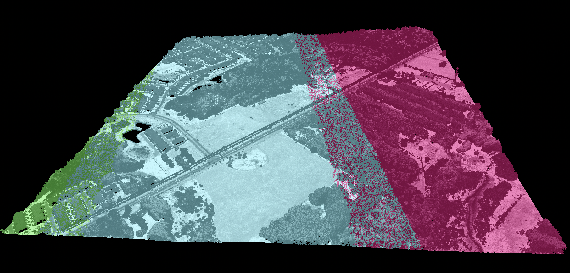
Please note that because this tool sorts points by their timestamps, the order of points in the output file may not match that of the input file.
See Also
flightline_overlap, find_flightline_edge_points, LidarSortByTime
Function Signature
def recover_flightline_info(self, input: Lidar, max_time_diff: float = 5.0, pt_src_id: bool = False, user_data: bool = False, rgb: bool = False) -> Lidar: ...
recreate_pass_lines
License Information
Use of this function requires a license for Whitebox Workflows for Python Professional (WbW-Pro). Please visit www.whiteboxgeo.com to purchase a license.
Description
This tool can be used to approximate the combine harvester swath pass lines from yield points. It is sometimes
the case that either pass-line information is not stored in the point data created during harvesting, or
that this information is lost. The yield_filter and yield_map tools however require information about the
associated swath path for each point in the dataset. This tool can therefore serve as a pre-processing
operation before running either of those more advanced mapping tools. It works by examining the geometry of
nearby points and associating points with line features that observe a maximum angular change in direction
(max_change_in_heading). The tool creates two output vectors, including a pass line vector (output) and
a points vector (output_points). The points output contains a PASS_NUM field within its attribute tables
that indicate the unique identifier associated with features. The line vector output contains an AVGYIELD
attribute field, which provides the pass-line average of the input yield values (yield_field_name).
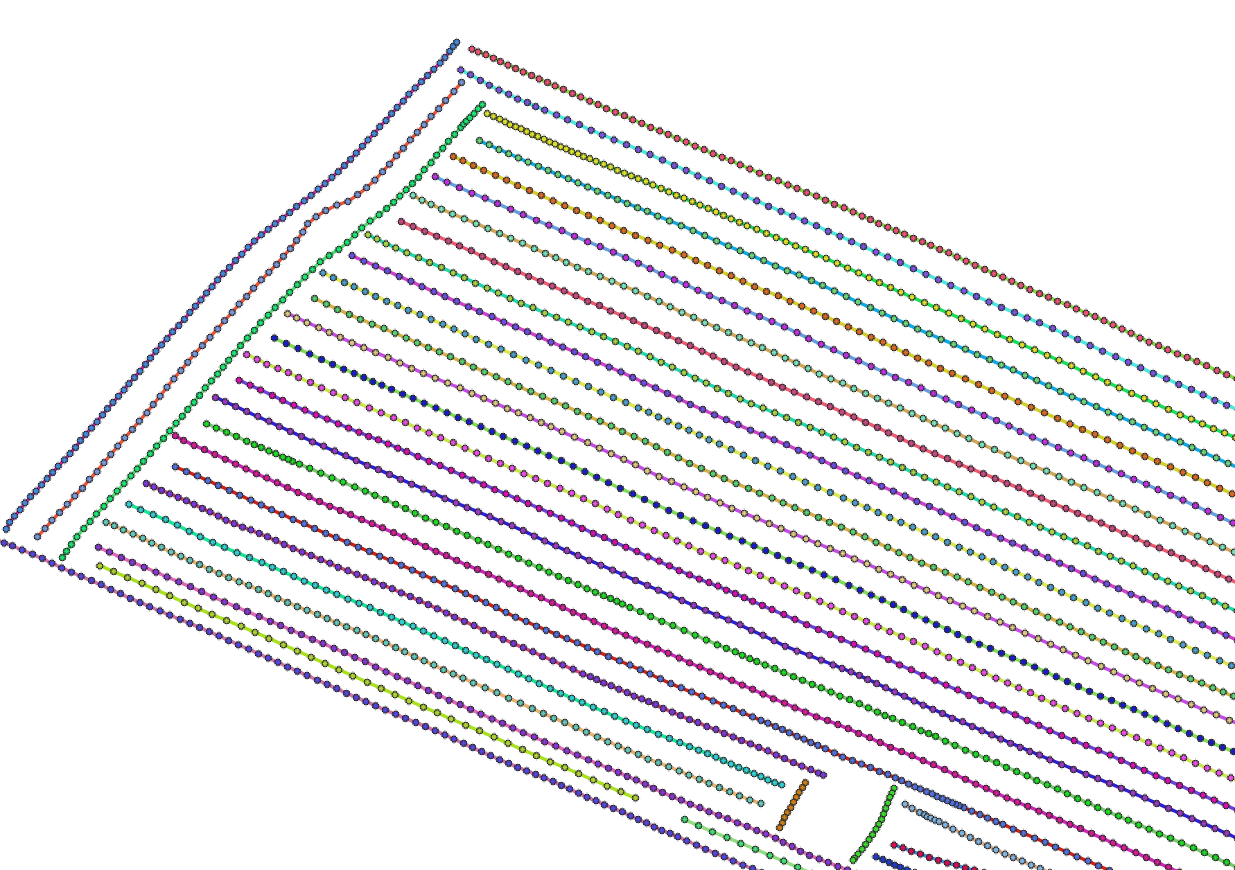
For a video tutorial on how to use the recreate_pass_lines, yield_filter and yield_map tools, see this YouTube video. There is also a blog that describes the usage of this tool on the WhiteboxTools homepage.
See Also
yield_filter, yield_map, reconcile_multiple_headers, remove_field_edge_points, yield_normalization
Function Signature
def recreate_pass_lines(self, input: Vector, yield_field_name: str, max_change_in_heading: float = 25.0, ignore_zeros: bool = False) -> Tuple[Vector, Vector]: ...
remove_field_edge_points
License Information
Use of this function requires a license for Whitebox Workflows for Python Professional (WbW-Pro). Please visit www.whiteboxgeo.com to purchase a license.
Description
This tool can be used to remove, or flag, most of the points along the edges from a crop yield data set. It is frequently the case that yield data collected along the edges of fields are anomalous in value compared with interior values. There are many reasons for this phenomenon, but one of the most common is that the header may be only partially full.
The user must specify the name of the input vector yield points data set (input), the output
points vector (output), the average distance between passes (dist), in meters, and the
maximum angular change in direction (max_change_in_heading), which is used to map pass lines
(see also recreate_pass_lines).
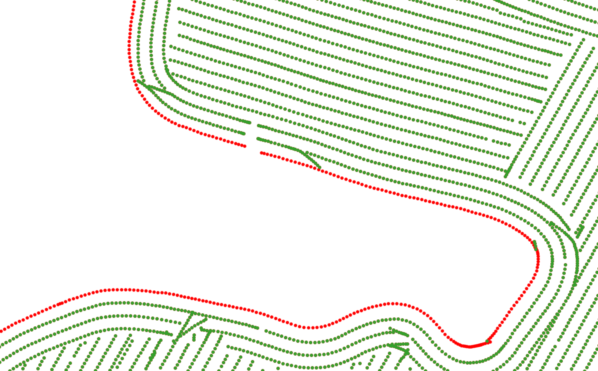
For a video tutorial on how to use the remove_field_edge_points tool, see this YouTube video.
See Also
yield_filter, reconcile_multiple_headers, yield_map, recreate_pass_lines, yield_normalization
Function Signature
def remove_field_edge_points(self, input: Vector, radius: float, max_change_in_heading: float = 25.0, flag_edges: bool = False) -> Vector: ...
remove_raster_polygon_holes
License Information
Use of this function requires a license for Whitebox Workflows for Python Professional (WbW-Pro). Please visit www.whiteboxgeo.com to purchase a license.
Description
This tool can be used to remove holes in raster polygons. Holes are areas of background values (either zero or
NoData), completely surrounded by foreground values (any value other than zero or NoData). Therefore, this tool can
somewhat be considered to be the raster equivalent to the vector-based remove_polygon_holes tool. Users may
optionally remove holes less than a specified threshold size (threshold), measured in grid cells. Hole size
is determined using a clumping operation, similar to what is used by the clump tool. Users may also optionally
specify whether or not to included 8-cell diagonal connectedness during the clumping operation (use_diagonals).
Some GIS professionals have previously used a closing operation to lessen the extent of polygon holes in raster data. A closing is a mathematical morphology operation that involves expanding the raster polygons using a dialation filter (maximum_filter), followed by a dialation filter (minimum_filter) on the resulting image. While this common image processing technique can be helpful for reducing the prevalance of polygon holes, it can also have considerable impact on non-hole features within the image. The remove_raster_polygon_holes tool, by comparison, will only affect hole features and does not impact the boundaries of other polygons at all. The following image compares the removal of polygon holes (islands in a lake polygon) using a closing operation (middle) calculated using an 11x11 convolution filter and the output of the remove_raster_polygon_holes tool. Notice how the convolution operation impacts the edges of the polygon, particularly in convex regions, compared with the remove_raster_polygon_holes.
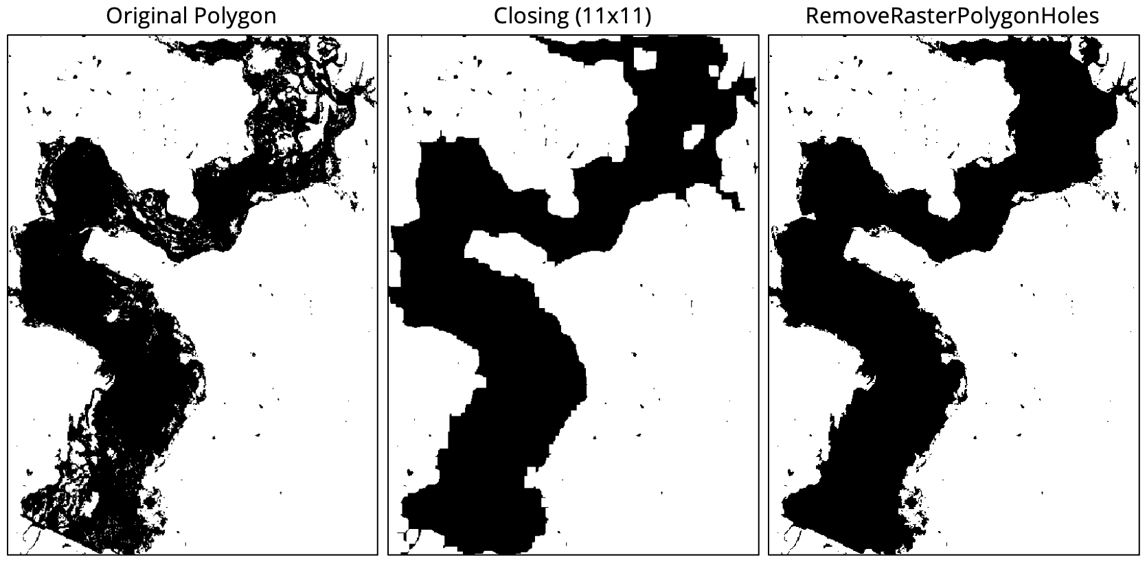
Here is a video that demonstrates how to apply this tool to a classified Sentinel-2 multi-spectral satellite imagery data set.
See Also
closing, remove_polygon_holes, clump, generalize_classified_raster
Function Signature
def remove_raster_polygon_holes(self, input: Raster, threshold_size: int = sys.maxsize, use_diagonals: bool = False) -> Raster: ...
ridge_and_valley_vectors
Use of this function requires a license for Whitebox Workflows for Python Professional (WbW-Pro). Please visit www.whiteboxgeo.com to purchase a license.
This function can be used to extract ridge and channel vectors from an input digital elevation model (DEM). The function works by first calculating elevation percentile (EP) from an input DEM using a neighbourhood size set by the user-specified filter_size parameter. Increasing the value of filter_size can result in more continuous mapped ridge and valley bottom networks. A thresholding operation is then applied to identify cells that have an EP less than the user-specified ep_threshold (valley bottom regions) and a second thresholding operation maps regions where EP is greater than 100 - ep_threshold (ridges). Each of these ridge and valley region maps are also multiplied by a slope mask created by identify all cells with a slope greater than the user-specified slope_threshold value, which is set to zero by default. This second thresholding can be helpful if the input DEM contains extensive flat areas, which can be confused for valleys otherwise. The filter_size and ep_threshold parameters are somewhat dependent on one another. Increasing the filter_size parameter generally requires also increasing the value of the ep_threshold. The ep_threshold can take values between 5.0 and 50.0, where larger values will generally result in more extensive and continuous mapped ridge and valley bottom networks. For many DEMs, a value on the higher end of the scale tends to work best.
After applying the thresholding operations, the function then applies specialized shape generalization, line thinning, and vectorization alorithms to produce the final ridge and valley vectors. The user must also specify the value of the min_length parameter, which determines the minimum size, in grid cells, of a mapped line feature. The function outputs a tuple of two vector, the first being the ridge network and the second vector being the valley-bottom network.
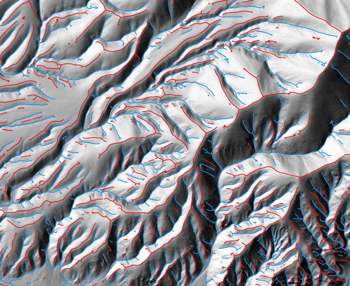
Code Example
from whitebox_workflows import WbEnvironment

# Set up the WbW environment
license_id = 'my-license-id' # Note, this tool requires a license for WbW-Pro
wbe = WbEnvironment(license_id)
try:
    wbe.verbose = True
    wbe.working_directory = '/path/to/data'

    # Read the input DEM
    dem = wbe.read_raster('DEM.tif')

    # Run the operation
    ridges, valleys = wbe.ridge_and_valley_vectors(dem, filter_size=21, ep_threshold=45.0, slope_threshold=1.0, min_length=25)
    wbe.write_vector(ridges, 'ridges_lines.shp')
    wbe.write_vector(valley, 'valley_lines.shp')

    print('Done!')
except Exception as e:
  print("Error: ", e)
finally:
    wbe.check_in_license(license_id)
See Also:
Function Signature
def ridge_and_valley_vectors(self, dem: Raster, filter_size: int = 11, ep_threshold: float = 30.0, slope_threshold: float = 0.0, min_length: int = 20) -> Tuple[Raster, Raster]:
ring_curvature
License Information
Use of this function requires a license for Whitebox Workflows for Python Professional (WbW-Pro). Please visit www.whiteboxgeo.com to purchase a license.
Description
This tool calculates the ring curvature, which is the product of horizontal excess and vertical excess curvatures (Shary, 1995), from a digital elevation model (DEM). Like rotor, ring curvature is used to measure flow line twisting. Ring curvature has values equal to or greater than zero and is measured in units of m-2.
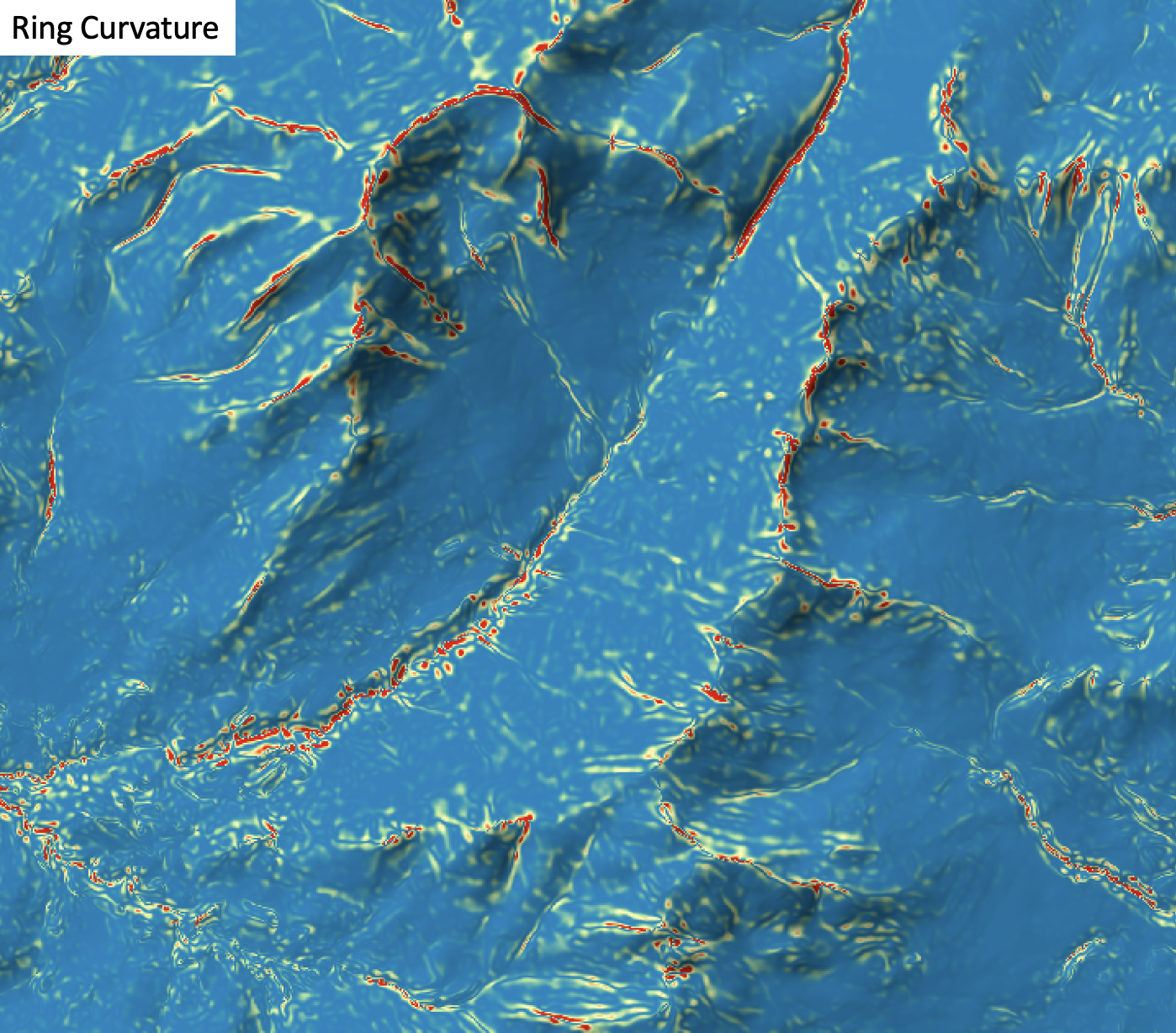
The user must specify the name of the input DEM (dem) and the output raster (output). The
The Z conversion factor (zfactor) is only important when the vertical and horizontal units are not the
same in the DEM. When this is the case, the algorithm will multiply each elevation in the DEM by the
Z Conversion Factor. Curvature values are often very small and as such the user may opt to log-transform
the output raster (log). Transforming the values applies the equation by Shary et al. (2002):
Θ' = sign(Θ) ln(1 + 10n|Θ|)
where Θ is the parameter value and n is dependent on the grid cell size.
For DEMs in projected coordinate systems, the tool uses the 3rd-order bivariate Taylor polynomial method described by Florinsky (2016). Based on a polynomial fit of the elevations within the 5x5 neighbourhood surrounding each cell, this method is considered more robust against outlier elevations (noise) than other methods. For DEMs in geographic coordinate systems (i.e. angular units), the tool uses the 3x3 polynomial fitting method for equal angle grids also described by Florinsky (2016).
References
Florinsky, I. (2016). Digital terrain analysis in soil science and geology. Academic Press.
Florinsky, I. V. (2017). An illustrated introduction to general geomorphometry. Progress in Physical Geography, 41(6), 723-752.
Shary PA (1995) Land surface in gravity points classification by a complete system of curvatures. Mathematical Geology 27: 373–390.
Shary P. A., Sharaya L. S. and Mitusov A. V. (2002) Fundamental quantitative methods of land surface analysis. Geoderma 107: 1–32.
See Also
rotor, minimal_curvature, maximal_curvature, mean_curvature, gaussian_curvature, profile_curvature, tangential_curvature
Function Signature
def ring_curvature(self, dem: Raster, log_transform: bool = False, z_factor: float = 1.0) -> Raster: ...
river_centerlines
Note this tool is part of a WhiteboxTools extension product. Please visit Whitebox Geospatial Inc. for information about purchasing a license activation key (https://www.whiteboxgeo.com/extension-pricing/).
This tool can map river centerlines, or medial-lines, from input river rasters (input). The input river (or
water) raster is often derived from an image classification performed on multispectral satellite imagery. The
river raster must be a Boolean (1 for water, 0/NoData for not-water) and can be derived either by reclassifying
the classification output, or derived using a 1-class classification procedure. For example, using the
parallelepiped_classification tool, it is possible to train the classifier using water training polygons,
and all other land classes will simply be left unclassified. It may be necessary to perform some pre-processing
on the water Boolean raster before input to the centerlines tool. For example, you may need to remove smaller
water polygons associated with small lakes and ponds, and you may want to remove small islands from the remaining
water features. This tool will often create a bifurcating vector path around islands within rivers, even if those
islands are a single-cell in size. The remove_raster_polygon_holes tool can be used to remove islands in the
water raster that are smaller than a user-specified size. The user must also specify the minimum line length
(min_length), which determines the level of detail in the final rivers map. For example, in the first iamge
below, a value of 30 grid cells was used for the min_length parameter, while a value of 5 was used in the
second image, which possesses far more (arguably too much) detail.
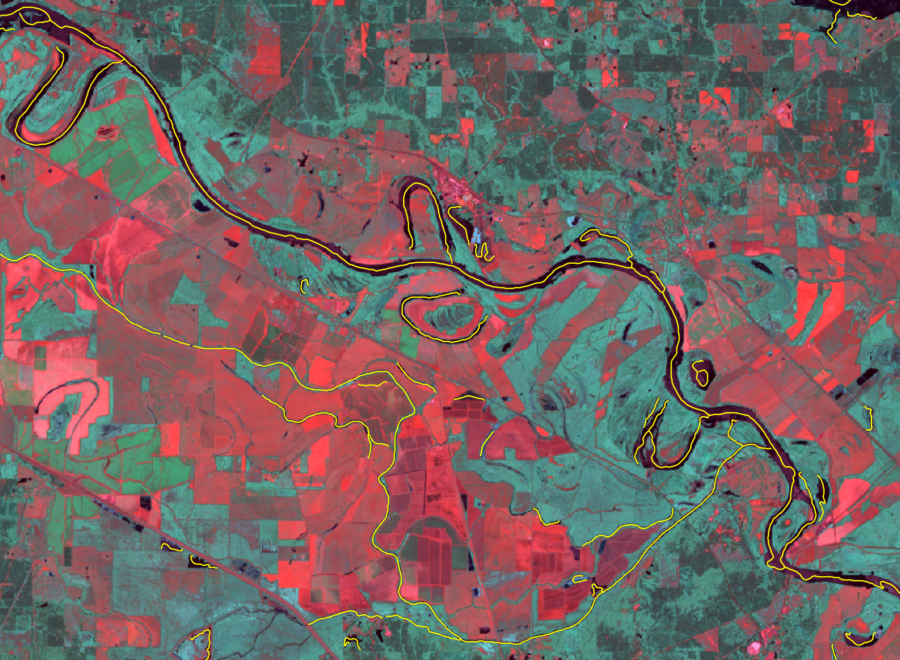
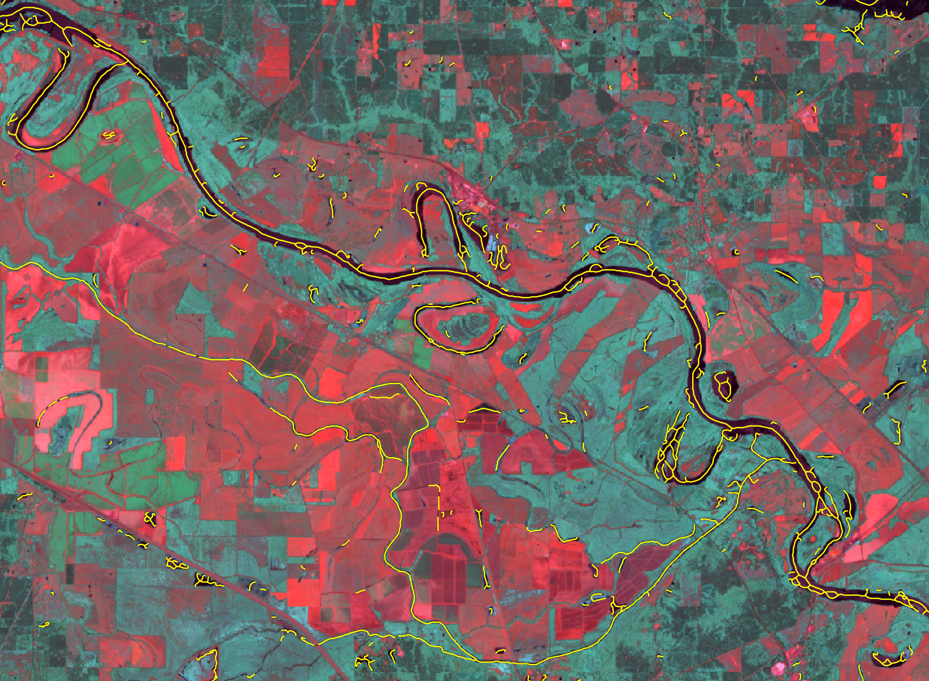
Lastly, the user must specify the radius parameter value. At times, the tool will be able to connect distant
water polygons that are part of the same feature and this parameter determines the size of the search radius
used to identify separated line end-nodes that are candidates for connection. It is advisable that this value
not be set too high, or else unexpected connections may be made between unrelated water features. However, a value
of between 1 and 5 can produce satisfactory results. Experimentation may be needed to find an appropriate value
for any one data set however. The image below provides an example of this characteristic of the tool, where
the resulting vector stream centerline passes through disconnected raster water polygons in the underlying input
image in four locations.
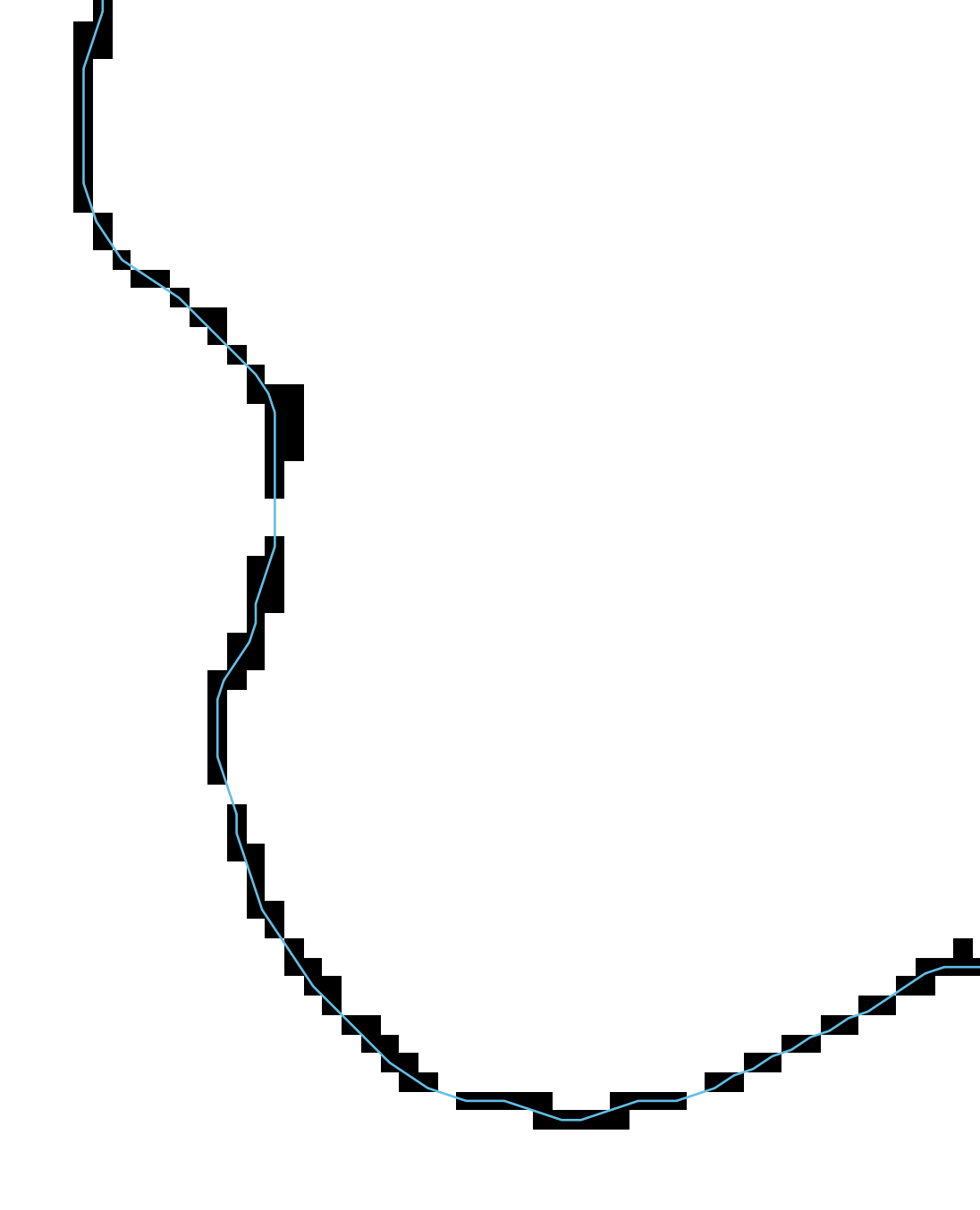
Here is a video that demonstrates how to apply this tool to map river center-lines taken from a water raster created by classifying a Sentinel-2 multi-spectral satellite imagery data set.
See Also
parallelepiped_classification, remove_raster_polygon_holes
Function Signature
def river_centerlines(self, raster: Raster, min_length: int = 3, search_radius: int = 9) -> Vector: ...
rotor
License Information
Use of this function requires a license for Whitebox Workflows for Python Professional (WbW-Pro). Please visit www.whiteboxgeo.com to purchase a license.
Description
This tool calculates the spatial pattern of rotor, which describes the degree to which a flow line twists (Shary, 1991), from a digital elevation model (DEM). Rotor has an unbounded range, with positive values indicating that a flow line turns clockwise and negative values indicating flow lines that turn counter clockwise (Florinsky, 2017). Rotor is measured in units of m-1.
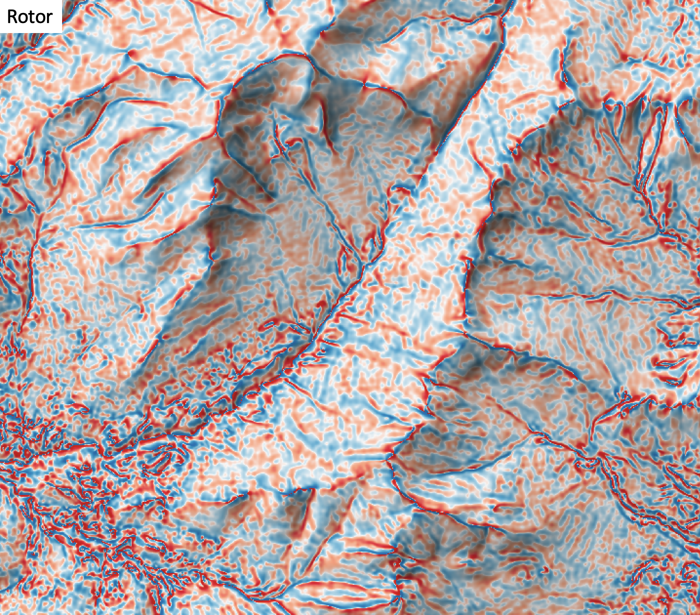
The user must specify the name of the input DEM (dem) and the output raster (output). The
The Z conversion factor (zfactor) is only important when the vertical and horizontal units are not the
same in the DEM. When this is the case, the algorithm will multiply each elevation in the DEM by the
Z Conversion Factor. Curvature values are often very small and as such the user may opt to log-transform
the output raster (log). Transforming the values applies the equation by Shary et al. (2002):
Θ' = sign(Θ) ln(1 + 10n|Θ|)
where Θ is the parameter value and n is dependent on the grid cell size.
For DEMs in projected coordinate systems, the tool uses the 3rd-order bivariate Taylor polynomial method described by Florinsky (2016). Based on a polynomial fit of the elevations within the 5x5 neighbourhood surrounding each cell, this method is considered more robust against outlier elevations (noise) than other methods. For DEMs in geographic coordinate systems (i.e. angular units), the tool uses the 3x3 polynomial fitting method for equal angle grids also described by Florinsky (2016).
References
Florinsky, I. (2016). Digital terrain analysis in soil science and geology. Academic Press.
Florinsky, I. V. (2017). An illustrated introduction to general geomorphometry. Progress in Physical Geography, 41(6), 723-752.
Shary PA (1991) The second derivative topographic method. In: Stepanov IN (ed) The Geometry of the Earth Surface Structures. Pushchino, USSR: Pushchino Research Centre Press, 30–60 (in Russian).
Shary P. A., Sharaya L. S. and Mitusov A. V. (2002) Fundamental quantitative methods of land surface analysis. Geoderma 107: 1–32.
See Also
ring_curvature, profile_curvature, tangential_curvature, plan_curvature, mean_curvature, gaussian_curvature, minimal_curvature, maximal_curvature
Function Signature
def rotor(self, dem: Raster, log_transform: bool = False, z_factor: float = 1.0) -> Raster: ...
shadow_animation
License Information
Use of this function requires a license for Whitebox Workflows for Python Professional (WbW-Pro). Please visit www.whiteboxgeo.com to purchase a license.
Description
This tool creates an interactive animated GIF of shadows based on an input digital surface model (DSM).
The shadow model is based on the modelled positions of the sun throughout a user-specified date (date)
sampling at a regular interval (interval), in minutes. Similar to the time_in_daylight tool, this
tool uses calculated horizon angle (horizon_angle) values and a solar position model to determine which
grid cells are located in shadow areas due to distant obsticles. The calculation of horizon angle, requires
the user input a maximum search distance parameter (max_dist).
The location parameter (location) should take the form Lat/Long/UTC-offset, e.g. 43.5448/-80.2482/-4/.
Note, the location need only be approximate; the postion of the central location of the input DSM raster
should suffice.
The output (output) of this tool is an HTML file, containing the interactive GIF animation. Users
are able to zoom and pan around the displayed DEV animation. The DSM may be rendered in one of several
available palettes (palette) suitable for visualization topography. The user must also
specify the image height (height) in the output file, the time delay (delay, in milliseconds) used
in the GIF animation, and an optional label (label), which will appear in the upper lefthand corner.
Note that the output is simply HTML, CSS, javascript code, and a GIF file, which can be readily embedded
in other documents.
Users should be aware that the outut GIF can be very large in size, depending on the size of the input DEM file. To reduce the file size of the output, it may be desirable to coarsen the input DEM resolution using image resampling (resample).
The following is an example of what the output of this tool looks like. Click the image for an interactive example.
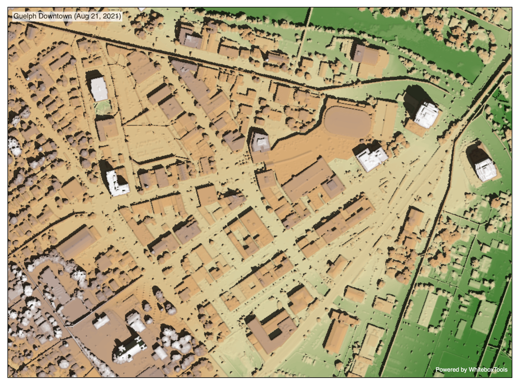
For more information about this tool, see this blog on the WhiteboxTools homepage.
See Also
shadow_image, time_in_daylight, horizon_angle, lidar_digital_surface_model
Function Signature
def shadow_animation(self, dem: Raster, output_html_file: str, palette: WbPalette = WbPalette.Soft, max_dist: float = float('inf'), date: str = "21/06/2021", time_interval: int = 30, location: str = "43.5448/-80.2482/-4", image_height: int = 600, delay: int = 250, label: str = "") -> None: ...
shadow_image
License Information
Use of this function requires a license for Whitebox Workflows for Python Professional (WbW-Pro). Please visit www.whiteboxgeo.com to purchase a license.
Description
This tool generates a raster of shadow areas based on an input digital surface model (DSM).
This shadow model is based on the calculated positions of the sun throughout a user-specified date (date),
sampling at a regular interval (interval), in minutes. Similar to the time_in_daylight tool, this
tool uses calculated horizon angle (horizon_angle) values and a solar position model to determine which
grid cells are located in shadow areas due to distant obsticles. The calculation of horizon angle, requires
the user input a maximum search distance parameter (max_dist).
The user must specify the date (date), time (time), and location (location) of the input DSM. The
date should have the format DD/MM/YYYY, e.g. 27/11/1976. The time should have the format HH::MM, e.g. 03:15AM
or 14:30. The location parameter should take the form Lat/Long/UTC-offset, e.g. 43.5448/-80.2482/-4/. Note, the
location need only be approximate; the postion of the central location of the input DSM raster should suffice.
The output (output) of this tool is a raster. If a palette (palette) is chosen, then the output
raster will be a colour composite image, containing a hysometrically tinted (i.e. elevation coloured)
shadow model. The DSM may be rendered in one of several available palettes (palette) suitable for
visualization topography. If the palette is set to 'none', the output image will not be a colour composite,
but rather, will be a 16-bit integer raster, and should be displayed in a grey-scale palette.
The following is an example of what the output of this tool looks like.
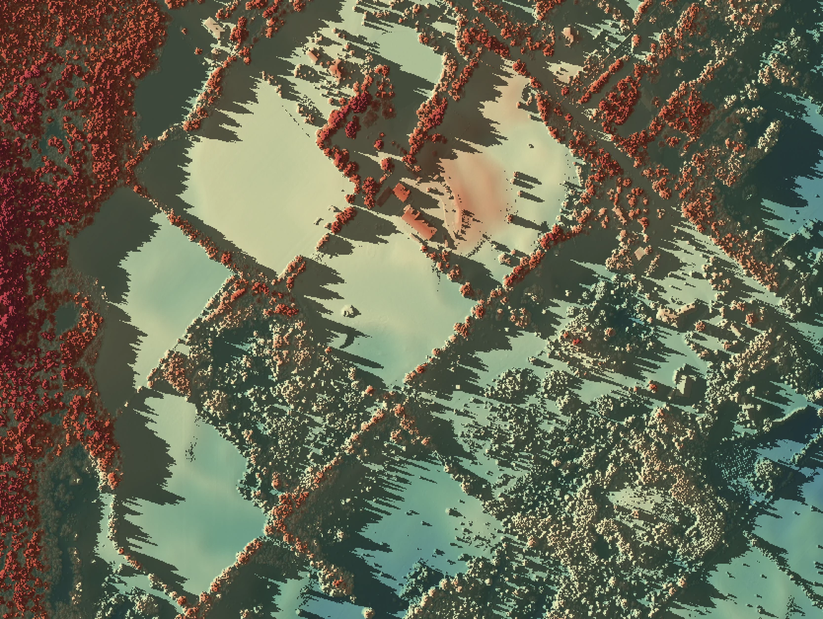
For more information about this tool, see this blog on the WhiteboxTools homepage.
See Also
shadow_animation, time_in_daylight, horizon_angle, lidar_digital_surface_model, hypsometrically_tinted_hillshade
Function Signature
def shadow_image(self, dem: Raster, palette: WbPalette = WbPalette.Soft, max_dist: float = float('inf'), date: str = "21/06/2021", time: str = "13:00", location: str = "43.5448/-80.2482/-4") -> Raster: ...
shape_index
License Information
Use of this function requires a license for Whitebox Workflows for Python Professional (WbW-Pro). Please visit www.whiteboxgeo.com to purchase a license.
Description
This tool calculates the shape index (Koenderink and van Doorn, 1992) from a digital elevation model (DEM). This variable ranges from -1 to 1, with positive values indicative of convex landforms, negative values corresponding to concave landforms (Florinsky, 2017). Absolute values from 0.5 to 1.0 are associated with elliptic surfaces (hills and closed depressions), while absolute values from 0.0 to 0.5 are typical of hyperbolic surface form (saddles). Shape index is a dimensionless variable and has utility in landform classification applications.
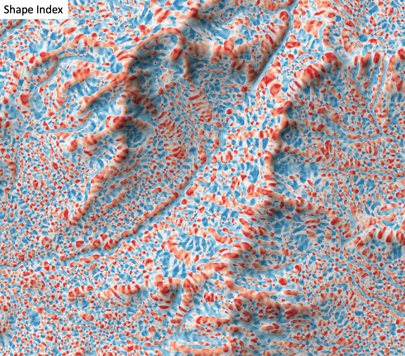
Koenderink and vsn Doorn (1992) make the following observations about the shape index:
-
Two shapes for which the shape index differs merely by sign represent complementary pairs that will fit together as ‘stamp’ and ‘mould’ when suitably scaled;
-
The shape for which the shape index vanishes - and consequently has indeterminate sign - represents the objects which are congruent to their own moulds;
-
Convexities and concavities find their places on opposite sides of the shape scale. These basic shapes are separated by those shapes which are neither convex nor concave, that are the saddle-like objects. The transitional shapes that divide the convexities/concavities from the saddle-shapes are the cylindrical ridge and the cylindrical rut.
The user must specify the name of the input DEM (dem) and the output raster (output). The
The Z conversion factor (zfactor) is only important when the vertical and horizontal units are not the
same in the DEM. When this is the case, the algorithm will multiply each elevation in the DEM by the
Z Conversion Factor.
For DEMs in projected coordinate systems, the tool uses the 3rd-order bivariate Taylor polynomial method described by Florinsky (2016). Based on a polynomial fit of the elevations within the 5x5 neighbourhood surrounding each cell, this method is considered more robust against outlier elevations (noise) than other methods. For DEMs in geographic coordinate systems (i.e. angular units), the tool uses the 3x3 polynomial fitting method for equal angle grids also described by Florinsky (2016).
References
Florinsky, I. (2016). Digital terrain analysis in soil science and geology. Academic Press.
Florinsky, I. V. (2017). An illustrated introduction to general geomorphometry. Progress in Physical Geography, 41(6), 723-752.
Koenderink, J. J., and Van Doorn, A. J. (1992). Surface shape and curvature scales. Image and vision computing, 10(8), 557-564.
curvedness, minimal_curvature, maximal_curvature, tangential_curvature, profile_curvature, mean_curvature, gaussian_curvature
Function Signature
def shape_index(self, dem: Raster, z_factor: float = 1.0) -> Raster: ...
sieve
Use of this function requires a license for Whitebox Workflows for Python Professional (WbW-Pro). Please visit www.whiteboxgeo.com to purchase a license.
The sieve function removes individual objects in a class map that are less than a threshold area, in grid cells. Pixels contained within the removed small polygons will be replaced with the nearest remaining class value. This operation is common when generalizing class maps, e.g. those derived from an image classification. Thus, this tool provides a similar function to the generalize_classified_raster and generalize_with_similarity functions.
See Also:
generalize_classified_raster, generalize_with_similarity
Function Signature
def sieve(self, input_raster: Raster, threshold: int = 1, zero_background: bool = False) -> Raster: ...
sky_view_factor
License Information
Use of this function requires a license for Whitebox Workflows for Python Professional (WbW-Pro). Please visit www.whiteboxgeo.com to purchase a license.
This tool calculates the sky-view factor (SVF) from an input digital elevation model (DEM) or digital surface model (DSM). The SVF is the proportion of the celestial hemisphere above a point on the earth's surface that is not obstructed by the surrounding land surface. It is often used to model the diffuse light that is received at the surface and has also been applied as a relief-shading technique (Böhner et al., 2009; Zakšek et al., 2011).
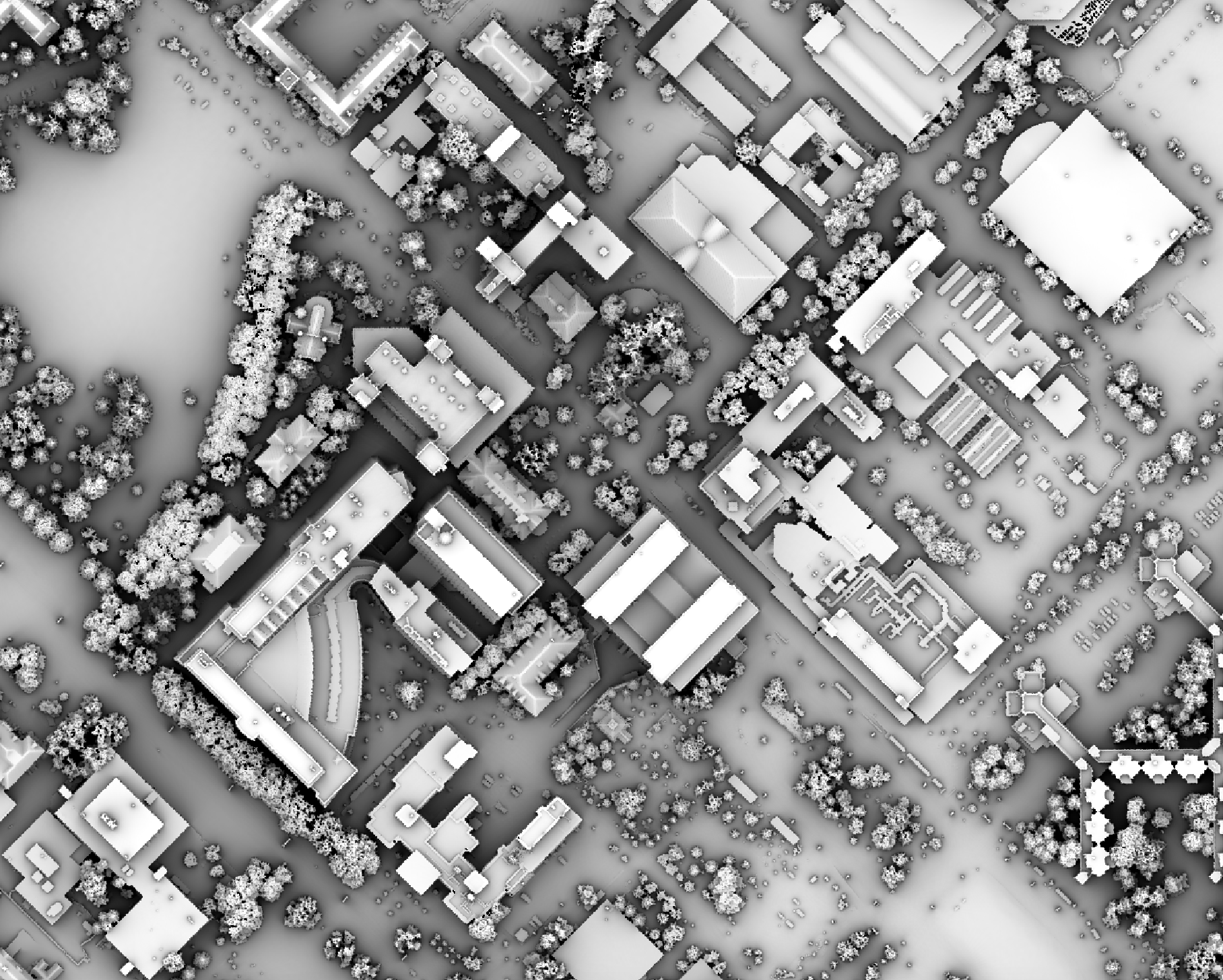
The user must specify an input DEM (dem), the azimuth fraction (az_fraction), the maximum search
distance (max_dist), and the height offset of the observer (observer_hgt_offset). The input DEM
should usually be a digital surface model (DSM) that contains significant off-terrain objects. Such a
model, for example, could be created using the first-return points of a LiDAR data set, or using the
lidar_digital_surface_model tool. The azimuth
fraction should be an even divisor of 360-degrees and must be between 1-45 degrees.
The tool operates by calculating horizon angle (see horizon_angle)
rasters from the DSM based on the user-specified azimuth fraction (az_fraction). For example, if an azimuth
fraction of 15-degrees is specified, horizon angle rasters would be calculated for the solar azimuths 0,
15, 30, 45... A horizon angle raster evaluates the vertical angle between each grid cell in a DSM and a
distant obstacle (e.g. a mountain ridge, building, tree, etc.) that obscures the view in a specified
direction. In calculating horizon angle, the user must specify the maximum search distance (max_dist),
in map units, beyond which the query for higher, more distant objects will cease. This parameter strongly
impacts the performance of the function, with larger values resulting in significantly longer processing-times.
This tool uses the method described by Zakšek et al. (2011) to calculate SVF, which differs slightly from the method described by Böhner et al. (2009), as implemented in the Saga software. Most notably the Whitebox implementation does not involve local surface slope gradient and is closer in definition to the Saga 'Visible Sky' index.
There are other significant differences between the Whitebox and Saga implementations of SVF. For a given
maximum search distance, the Whitebox SVF will be substantially faster to calculate. Furthermore, the
Whitebox implementation has the ability to specify a height offset of the observer from the ground
surface, using the observer_hgt_offset parameter. For example, the following image shows the spatial
pattern derived from a LiDAR DSM using observer_hgt_offset = 0.0:

Notice that there are several places, plarticularly on the flatter rooftops, where the local noise in the LiDAR DEM, associated with the individual scan lines, has resulted in a somewhat noisy pattern in the output. By adding a small height offset of the scale of this noise variation (0.15 m), we see that most of this noisy pattern is removed in the output below:
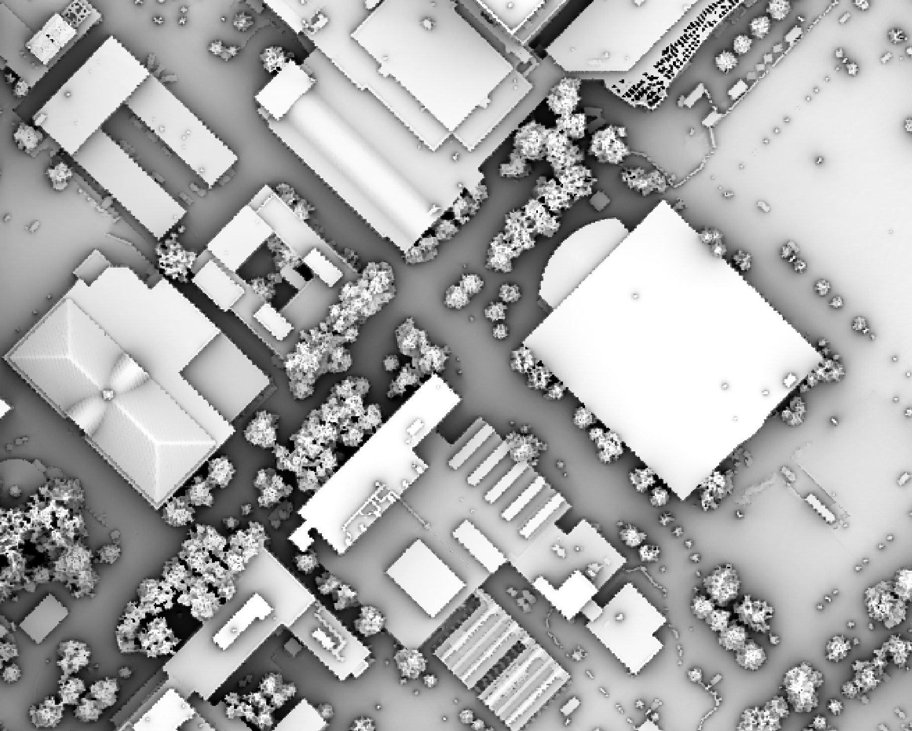
This feature makes the function more robust against DEM noise. As another example of the usefulness of
this additional parameter, in the image below, the observer_hgt_offset parameter has been used to
measure the pattern of the index at a typical human height (1.7 m):
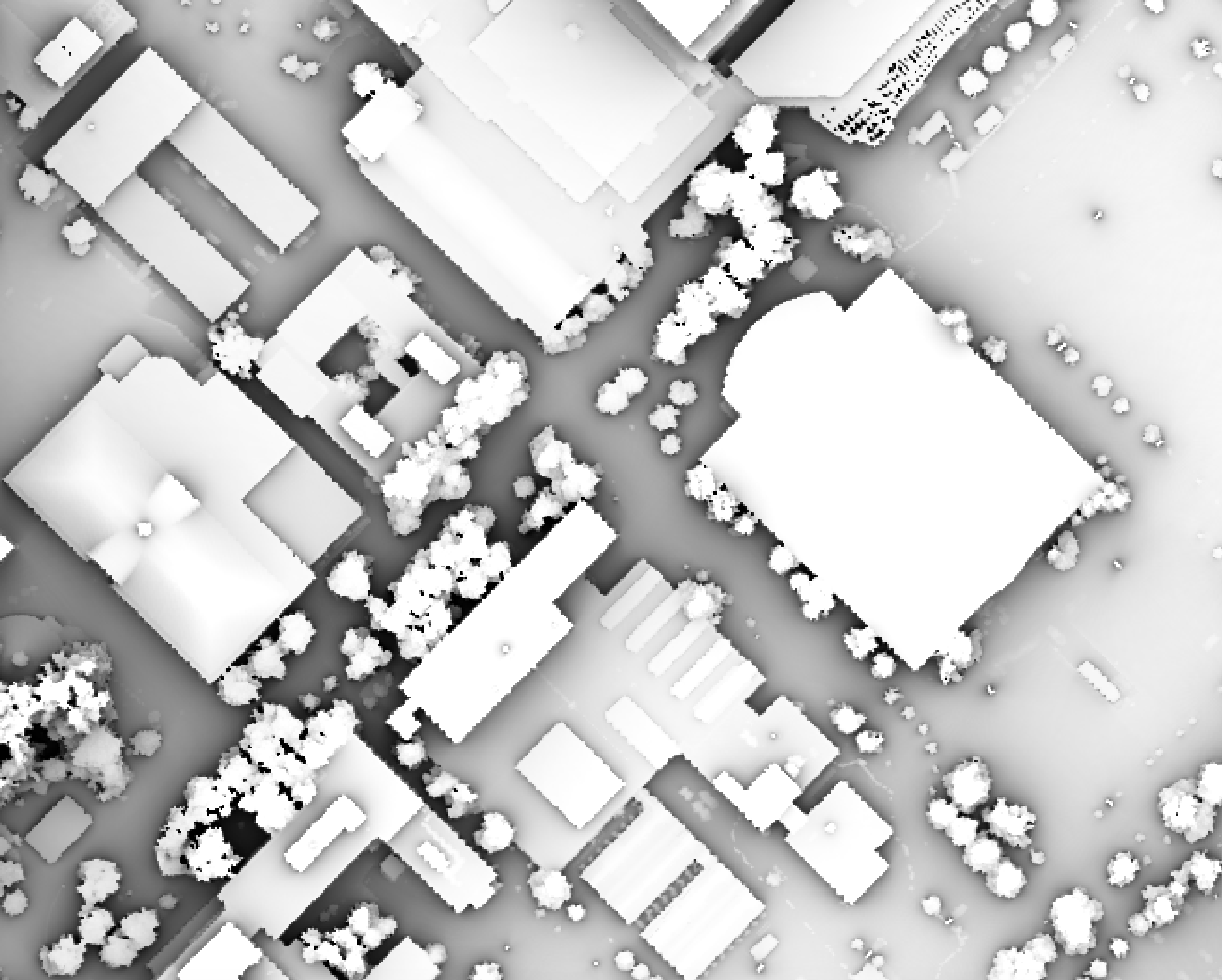
Notice how overall visiblility increases at this height.
References
Böhner, J. and Antonić, O., 2009. Land-surface parameters specific to topo-climatology. Developments in soil science, 33, pp.195-226.
Zakšek, K., Oštir, K. and Kokalj, Ž., 2011. Sky-view factor as a relief visualization technique. Remote sensing, 3(2), pp.398-415.
See Also
average_horizon_distance, horizon_area, openness, lidar_digital_surface_model, horizon_angle
Function Signature
def sky_view_factor(self, dem: Raster, az_fraction: float = 5.0, max_dist: float = float('inf'), observer_hgt_offset: float = 0.0) -> Raster: ...
skyline_analysis
License Information
Use of this function requires a license for Whitebox Workflows for Python Professional (WbW-Pro). Please visit www.whiteboxgeo.com to purchase a license.
This function performs a skyline analysis for one or more observation points based on the terrain of an underlying digital elevation model (DEM). There are two outputs of the analysis, including an HTML report and a vector containing the horizon polygons associated with each observation point. The analysis report includes a summary of key characteristics of the skyline for each point, including the average zenith angle, the average horizon distance, the horizon area, the average skyline elevation, the standard deviation of skyline elevation, and the sky-view factor. The report will also include two radial charts, including the zenith angle plot and the horizon distance plot, for each observation point.
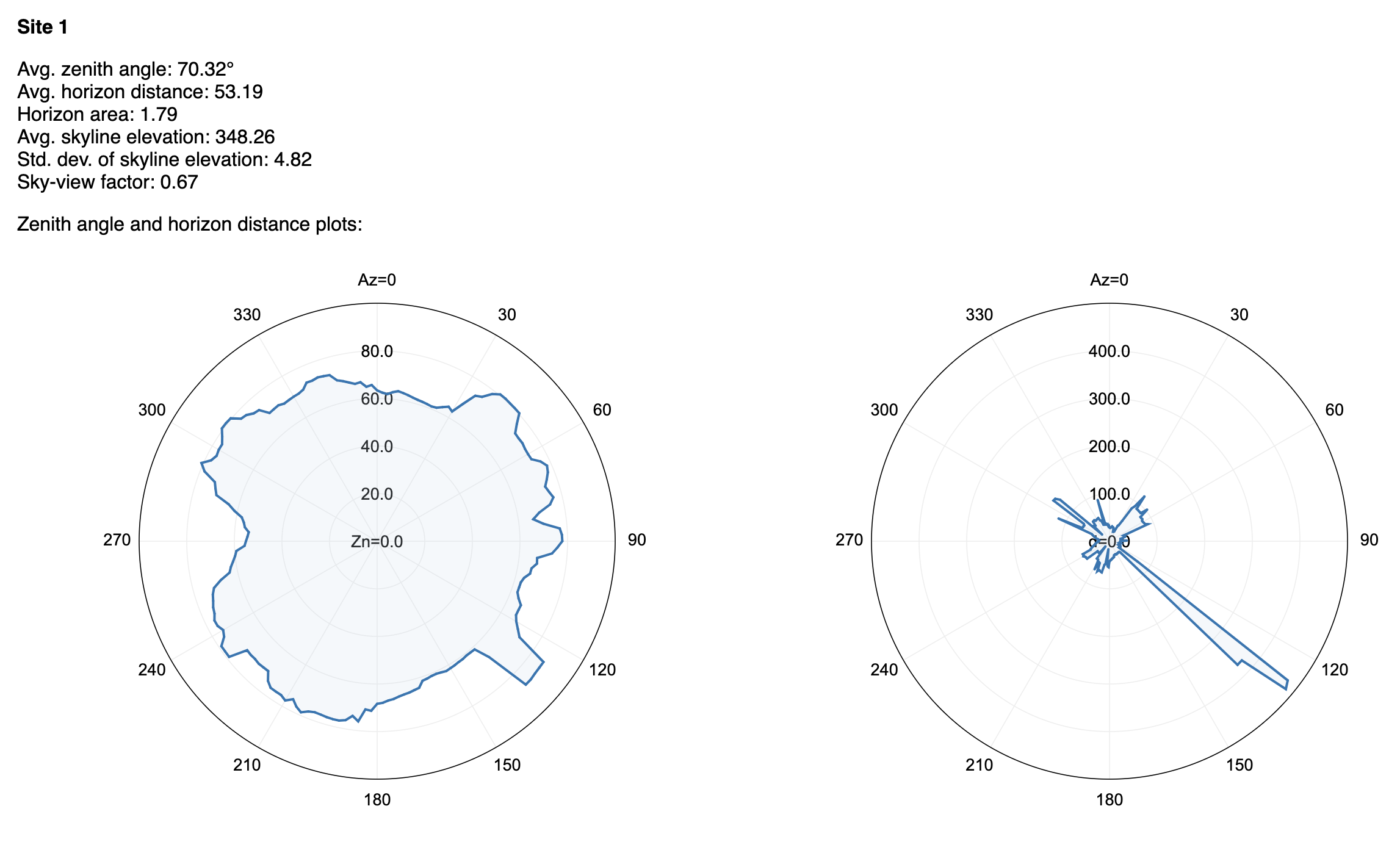
The horizon area vector output traces the skyline and is saved as a PolygonZ shapetype, with z-values taken from the input DEM surface and measures (M-values) derived from the zenith angle values. This can be thought of as an approxiate vector viewshed for the observation points, except that a viewshed may well contain internal occlusions that the horizon polygon does not. Note that it is best to use an input digital surface model, rather than a bare-earth DEM for this function.
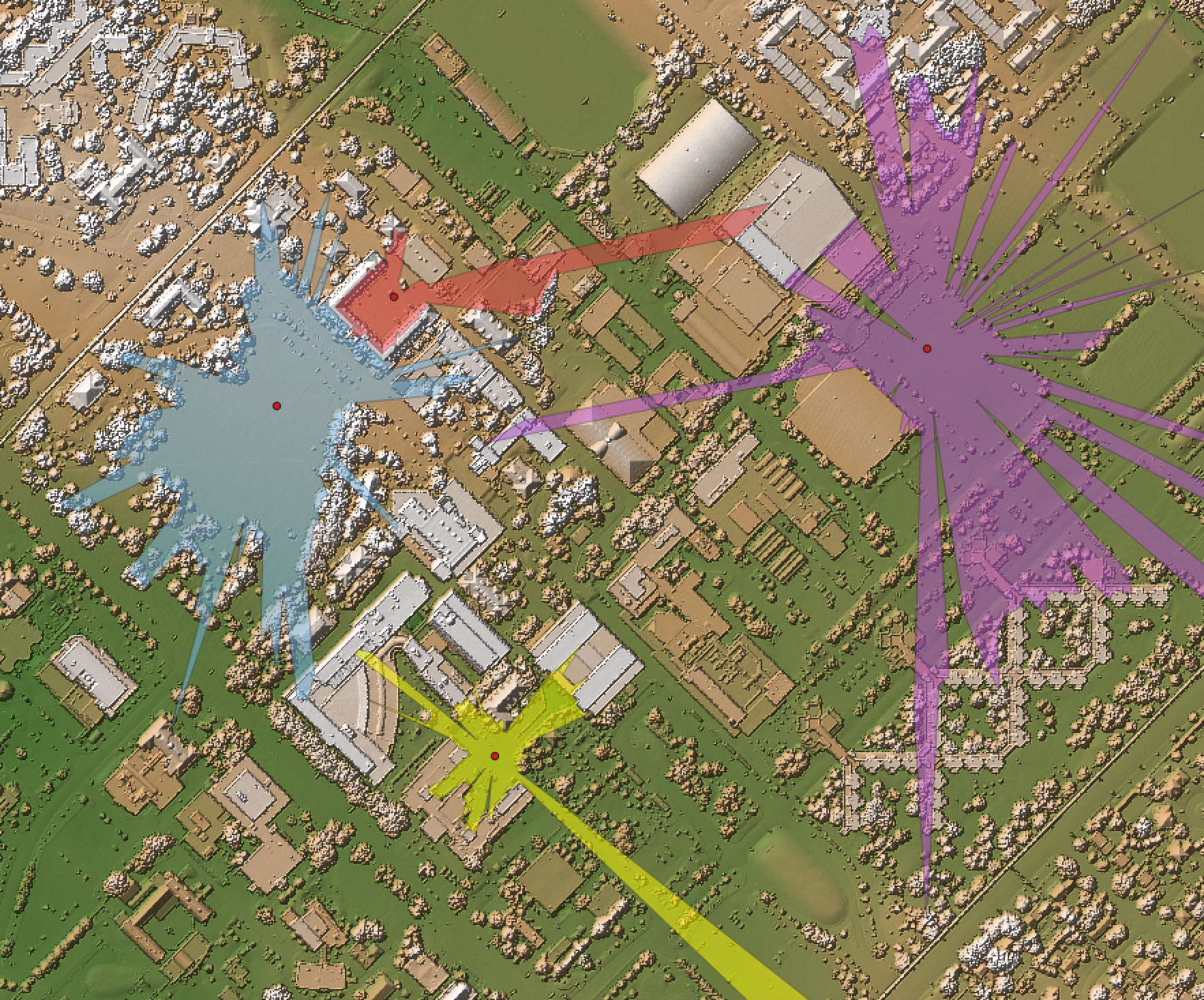
The user must specify the input DEM and vector points file, the name of the output HTML report (which will be automatically displayed if verbose=True), the maximum distance (max_dist), the observer height (observer_hgt_offset), whether the output horizon polygon should of the PolygonZ ShapeType (if set to False the output will be of the PolyLineZ ShapeType), and the azimuth fraction (az_fraction), which determines the angular resolution of the analysis, with a default value of 1.0.
Note that the input DEM should use a projected spatial referencing system.
See Also
sky_view_factor, average_horizon_distance, openness, lidar_digital_surface_model, horizon_angle
Function Signature
def skyline_analysis(self, dem: Raster, points: Vector, output_html_file: str, max_dist: float = float('inf'), observer_hgt_offset: float = 0.0, output_as_polygons: bool = True, az_fraction: float = 1.0) -> Vector: ...
slope_vs_aspect_plot
License Information
Use of this function requires a license for Whitebox Workflows for Python Professional (WbW-Pro). Please visit www.whiteboxgeo.com to purchase a license.
Description
This tool creates a slope vs. aspect plot for an input digital elevation model, or DEM (input).
Similar to a slope vs. elevation analysis (SlopeVsElevationPlot), the slope-aspect relation can reveal the basic
topographic character of a site. The output of this analysis is an HTML document (output) that contains the
slope-aspect chart, which is a radial line plot. The plot displays the median and interquartile range
of slope values for the range of aspect values from 0 - 360 degrees. In reality, the aspect range is binned
and the user must specify the bin size (bin_size). As slopes becomes quite shallow, the numerical
instability in aspect becomes apparent, due to the relatively small signal-to-noise ratio in these
areas of the input DEM. These shallow-gradient grid cells can have an out-sized impact on the shape
of the slope-aspect relation. Therefore, users can specify to ignore slopes less than a certain
threshold minimum slope (min_slope).
In interpreting the slope-aspect plots output by this tool, users should take note of asymmetries in polygonal paths taken by the percentile slope values, asymmetries in the range of slopes (i.e. the interquartile range), and anisotropy patterns (i.e. non-circularity or oval-shaped patterns). For example, asymmetries in the patterns may be indicative of landscape processes of interest, such as the differential energy balances experienced by north- and south-facing slopes at high latitudes. Increased rates of weathering on slopes with more direct sunlight at higher latitudes can result in flatter hillslopes. Asymmetry in the slope-aspect relation may also be indicative of DEM error and can be used as a quality control procedure, particularly for InSAR DEMs. Anisotropy in the slope-aspect relation may indicate a characteristic of the bedrock geology or the drainage structure of the landscape. The tool will also output the elongation ratio, a measure of anisotropy, of the mapped percentile polygons in a table.
The following are some examples of the output plots. In actuality, the outputs of the tool are interactive plots.
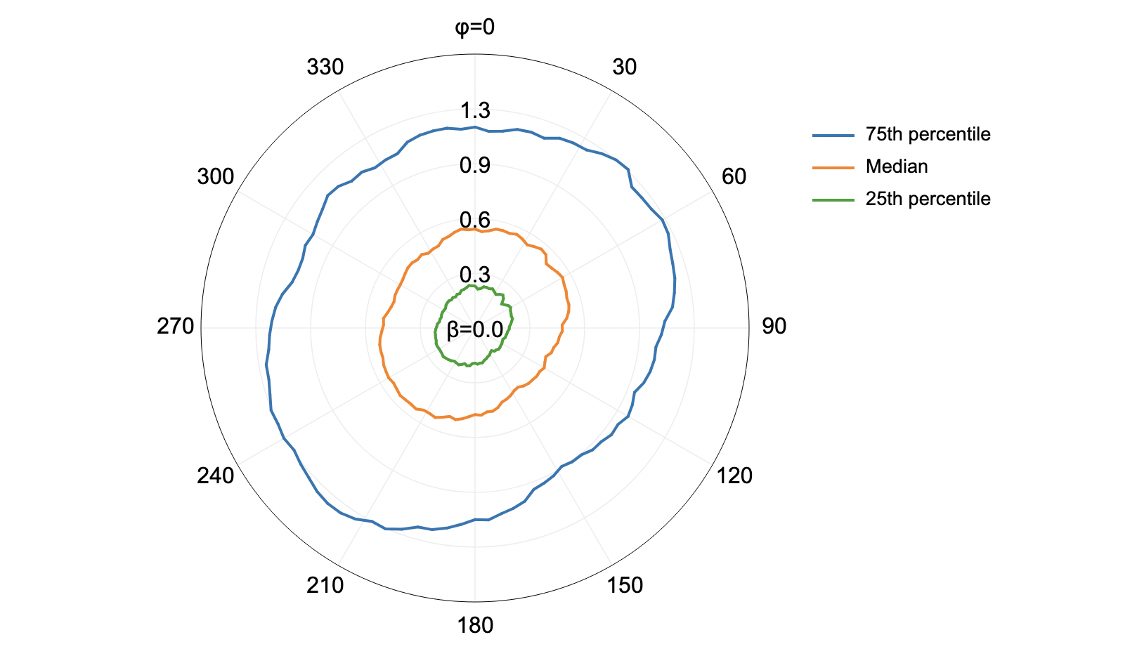
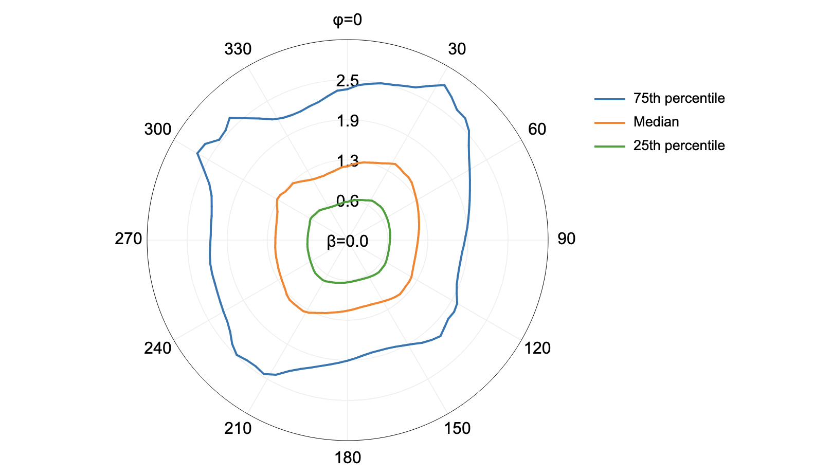
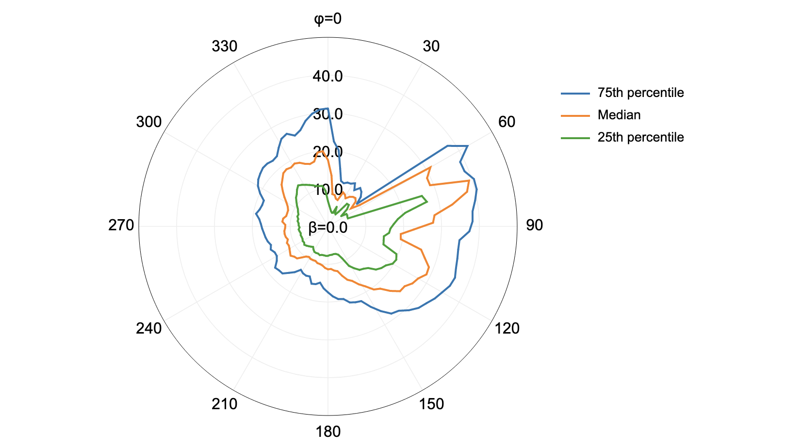
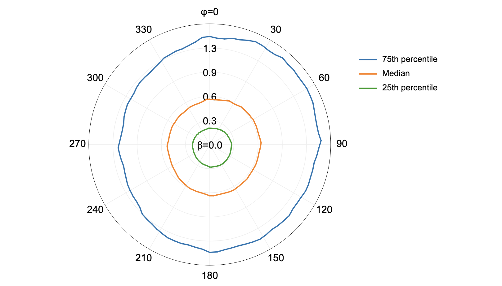
You may wish to smooth your DEM prior to analysis with this tool, in order to emphasis longer-scale patterns in the landscape. We would recommend using a method such as the feature_preserving_smoothing tool for this purpose.
The Z conversion factor (z_factor) is only important when the vertical and horizontal units are
not the same in the DEM. When this is the case, the algorithm will multiply each elevation in the
DEM by the Z conversion factor. If the DEM is in the geographic coordinate system (latitude and
longitude), the following equation is used:
zfactor = 1.0 / (111320.0 x cos(mid_lat))
where mid_lat is the latitude of the centre of each raster row, in radians.
See Also
SlopeVsElevationPlot, feature_preserving_smoothing
Function Signature
def slope_vs_aspect_plot(self, dem: Raster, output_html_file: str, aspect_bin_size: float = 2.0, min_slope: float = 0.1, z_factor: float = 1.0) -> None: ...
smooth_vegetation_residual
License Information
Use of this function requires a license for Whitebox Workflows for Python Professional (WbW-Pro). Please visit www.whiteboxgeo.com to purchase a license.
Description
This tool can smooth the roughness due to residual vegetation cover in LiDAR digital elevation models (DEMs).
Sometimes when LiDAR data are collected under heavy forest cover, particularly conifer species, the DEM
will contain substantial roughness, even if it is interpolated using last-return points only. This tool can
be used to reduce the roughness of the ground surface under these conditions. It works by identifying grid cells
that possess deviation in mean elevation (DEV, DevFromMeanElev) values that are higher than a specified
threshold value (dev_threshold) for tested scales less than a specified threshold (scale_threshold).
DEV is measured for the input DEM (input) using filter radii from 1 to a user-specified maximum (max_scale).
The identified grid cells are then masked out and their elevations are re-interpolated using the surrounding,
non-masked values.
This method can work well under some conditions, and will further benefit from multiple passes of the tool, i.e.
run the tool using one set of parameters and then use the output (output) as the input for the second pass.
Alternative approaches include use of the remove_off_terrain_objects tool, using low-pass filters such as the
feature_preserving_smoothing tool, or, if the point-cloud source data are available, classifying the ground
points using lidar_ground_point_filter and excluding non-ground points from the interpolation.
The following image shows an image of a DEM that is badly impacted by heavy forest cover, with obvious vegetation residual roughness.
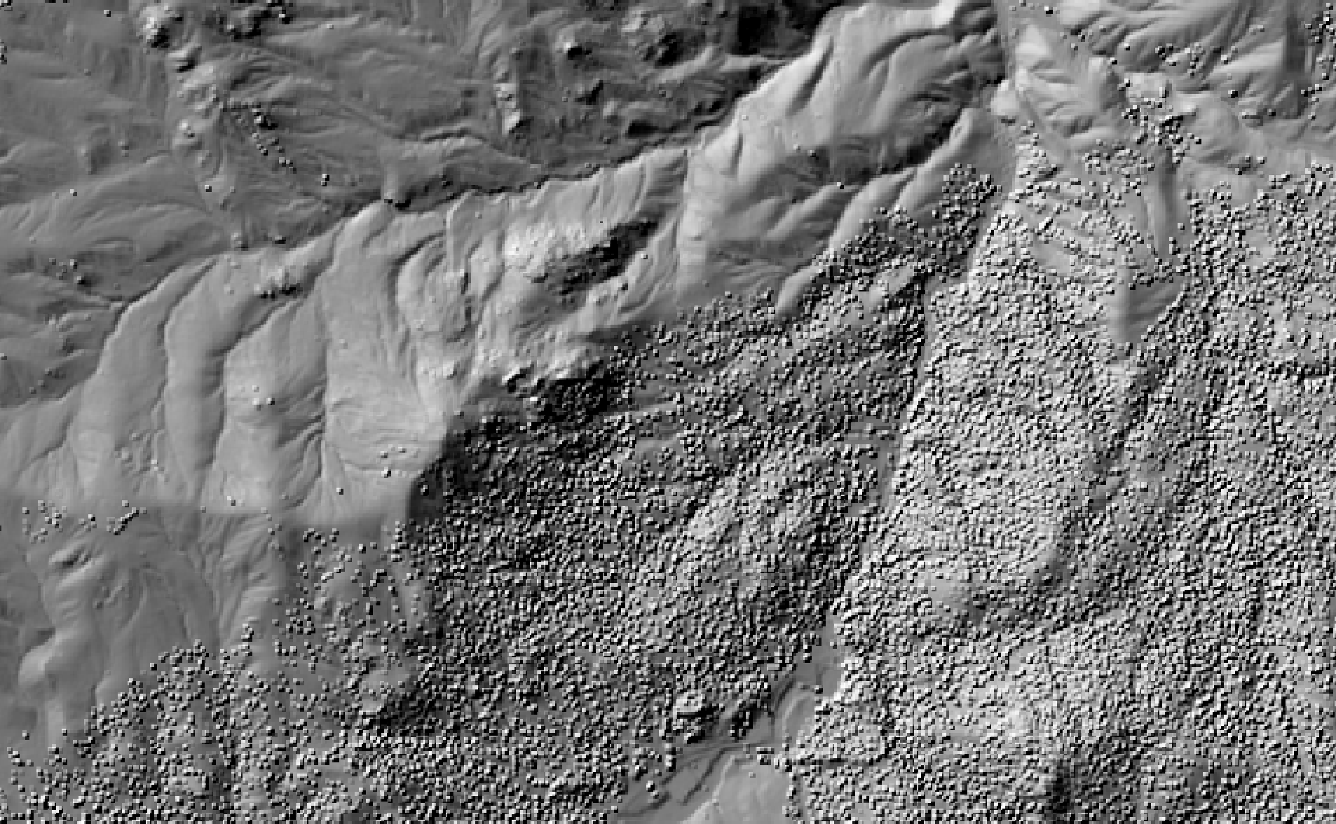
This image shows the impact of two-passes of the smooth_vegetation_residual tool.
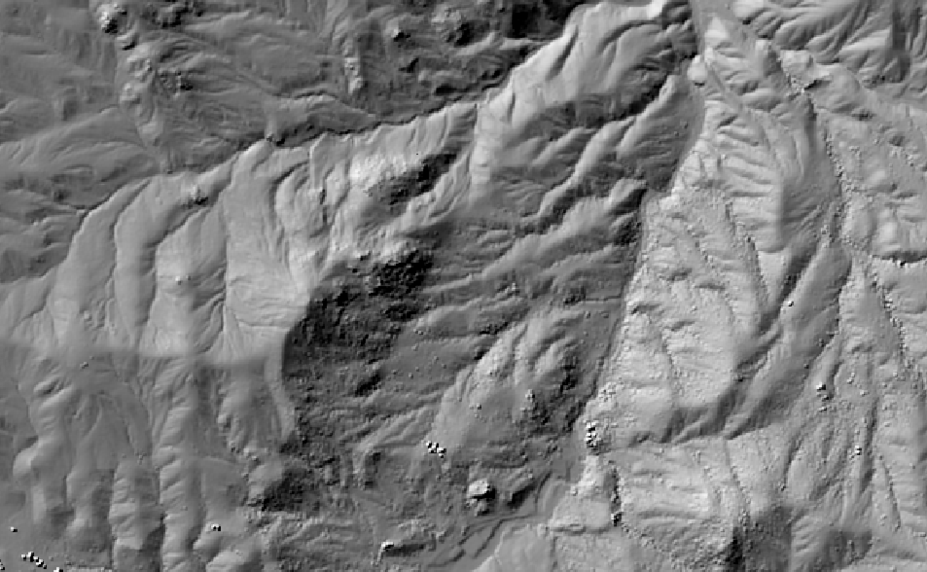
See Also
remove_off_terrain_objects, feature_preserving_smoothing, lidar_ground_point_filter, DevFromMeanElev
Function Signature
def smooth_vegetation_residual(self, dem: Raster, max_scale: int = 1, dev_threshold: float = 1.0, scale_threshold: int = 5) -> Raster: ...
sort_lidar
License Information
Use of this function requires a license for Whitebox Workflows for Python Professional (WbW-Pro). Please visit www.whiteboxgeo.com to purchase a license.
Description
This tool can be used to sort the points in an input LiDAR file (input) based on their properties
with respect to one or more sorting criteria (criteria). The sorting criteria may include: the x, y or z
coordinates (x, y, z), the intensity data (intensity), the point class value (class), the point
user data field (user_data), the return number (ret_num), the point source ID (point_source_id), the
point scan angle data (scan_angle), the scanner channel (scanner_channel; LAS 1.4 datasets only), and
the acquisition time (time). The following is an example of a complex sorting criteria statement that
includes multiple criteria:
x 100.0, y 100.0, z 10.0, scan_angle
Criteria should be separated by a comma, semicolon, or pipe (|). Each criteria may have an associated bin value.
In the example above, point x values are sorted into bins of 100 m, which are then sorted by y values into bins
of 100 m, and sorted by point z values into bins of 10 m, and finally sorted by their scan_angle.
Sorting point values can have a significant impact on the compression rate when using certain compressed LiDAR data formats (e.g. LAZ, zLidar). Sorting values can also improve the visualization speed in some rendering software.
Note that if the user does not specify the optional input LiDAR file, the tool will search for all valid LiDAR (*.las, *.laz, *.zlidar) files contained within the current working directory. This feature can be useful for processing a large number of LiDAR files in batch mode. When this batch mode is applied, the output file names will be the same as the input file names but with a '_sorted' suffix added to the end.
Function Signature
def sort_lidar(self, sort_criteria: str, input_lidar: Optional[Lidar]) -> Optional[Lidar]: ...
split_lidar
License Information
Use of this function requires a license for Whitebox Workflows for Python Professional (WbW-Pro). Please visit www.whiteboxgeo.com to purchase a license.
Description
This tool can be used to split an input LiDAR file (input) into a series of output files, placing
points into each output based on their properties with respect to a grouping criterion (criterion).
Points can be grouped based on a specified the number of points in the output file (num_pts; note
the last file may contain fewer points), the x, y or z coordinates (x, y, z), the intensity data
(intensity), the point class value (class), the point user data field (user_data), the
point source ID (point_source_id), the point scan angle data (scan_angle), and the acquisition time
(time). Points are binned into groupings based on a user-specified interval value (interval). For
example, if an interval of 50.0 is used with the z criterion, a series of files will be output that
are elevation bands of 50 m. The user may also optionally specify the minimum number of points needed before
a particular grouping file is saved (min_pts). The interval value is not used for the class and
point_source_id criteria.
With this tool, a single input file can generate many output files. The names of the output files will be
reflective of the point attribute used for the grouping and the bin. For example, running the tool with the
on an input file named my_file.las using intensity criterion and with an interval of 1000 may produce the
following files:
- my_file_intensity0.las
- my_file_intensity1000.las
- my_file_intensity2000.las
- my_file_intensity3000.las
- my_file_intensity4000.las
Where the number after the attribute (intensity, in this case) reflects the lower boundary of the bin. Thus, the first file contains all of the input points with intensity values from 0 to just less than 1000.
Note that if the user does not specify the optional input LiDAR file, the tool will search for all valid LiDAR (*.las, *.laz, *.zlidar) files contained within the current working directory. This feature can be useful for processing a large number of LiDAR files in batch mode. When this batch mode is applied, the output file names will be the same as the input file names but with a suffix added to the end reflective of the split criterion and value (see above).
See Also
sort_lidar, filter_lidar, modify_lidar, lidar_elevation_slice
Function Signature
def split_lidar(self, split_criterion: str, input_lidar: Optional[Lidar], interval: float = 5.0, min_pts: int = 5) -> None: ...
svm_classification
License Information
Use of this function requires a license for Whitebox Workflows for Python Professional (WbW-Pro). Please visit www.whiteboxgeo.com to purchase a license.
Description
This tool performs a support vector machine (SVM) binary classification
using multiple predictor rasters (inputs), or features, and training data (training). SVMs
are a common class of supervised learning algorithms widely applied in many problem domains. This
tool can be used to model the spatial distribution of class data, such as land-cover type, soil class, or vegetation type.
The training data take the form of an input vector Shapefile containing a set of points or polygons, for which the known
class information is contained within a field (field) of the attribute table. Each grid cell defines
a stack of feature values (one value for each input raster), which serves as a point within the
multi-dimensional feature space. Note that the svm_regression tool can be used to apply the SVM method
to the modelling of continuous data.
The user must specify the values of three parameters used in the development of the model, the c
parameters (-c), gamma (gamma), and the tolerance (tolerance). The c-value is the
regularization parameter used in model optimization. The gamma parameter defines the radial basis function
(Gaussian) kernel parameter. The tolerance parameter controls the stopping condition used during model
optimization.
The tool splits the training data into two sets, one for training the classifier and one for testing
the classification. These test data are used to calculate the overall accuracy and Matthew correlation
coefficient (MCC). The test_proportion parameter
is used to set the proportion of the input training data used in model testing. For example, if
test_proportion = 0.2, 20% of the training data will be set aside for testing, and this subset
will be selected randomly. As a result of this random selection of test data, the tool behaves stochastically,
and will result in a different model each time it is run.
Note that the output image parameter (output) is optional. When unspecified, the tool will simply
report the model accuracy statistics, allowing the user to experiment with different parameter
settings and input predictor raster combinations to optimize the model before applying it to classify
the whole image data set.
Like all supervised classification methods, this technique relies heavily on proper selection of training data. Training sites are exemplar areas/points of known and representative class value (e.g. land cover type). The algorithm determines the feature signatures of the pixels within each training area. In selecting training sites, care should be taken to ensure that they cover the full range of variability within each class. Otherwise the classification accuracy will be impacted. If possible, multiple training sites should be selected for each class. It is also advisable to avoid areas near the edges of class objects (e.g. land-cover patches), where mixed pixels may impact the purity of training site values.
After selecting training sites, the feature value distributions of each class type can be assessed using the evaluate_training_sites tool. In particular, the distribution of class values should ideally be non-overlapping in at least one feature dimension.
The SVM algorithm is based on the calculation of distances in multi-dimensional space. Feature scaling is
essential to the application of SVM-based modelling, especially when the ranges of the features are different, for
example, if they are measured in different units. Without scaling, features with larger ranges will have
greater influence in computing the distances between points. The tool offers three options for feature-scaling (scaling),
including 'None', 'Normalize', and 'Standardize'. Normalization simply rescales each of the features onto
a 0-1 range. This is a good option for most applications, but it is highly sensitive to outliers because
it is determined by the range of the minimum and maximum values. Standardization
rescales predictors using their means and standard deviations, transforming the data into z-scores. This
is a better option than normalization when you know that the data contain outlier values; however, it does
does assume that the feature data are somewhat normally distributed, or are at least symmetrical in
distribution.
Because the SVM algorithm calculates distances in feature-space, like many other related algorithms, it suffers from the curse of dimensionality. Distances become less meaningful in high-dimensional space because the vastness of these spaces means that distances between points are less significant (more similar). As such, if the predictor list includes insignificant or highly correlated variables, it is advisable to exclude these features during the model-building phase, or to use a dimension reduction technique such as principal_component_analysis to transform the features into a smaller set of uncorrelated predictors.
See Also
random_forest_classification, knn_classification, parallelepiped_classification, evaluate_training_sites, principal_component_analysis
Function Signature
def svm_classification(self, input_rasters: List[Raster], training_data: Vector, class_field_name: str, scaling_method: str = "none", c_value: float = 50.0, kernel_gamma: float = 0.5, tolerance: float = 0.1, test_proportion: float = 0.2, create_output: bool = False) -> Optional[Raster]: ...
svm_regression
License Information
Use of this function requires a license for Whitebox Workflows for Python Professional (WbW-Pro). Please visit www.whiteboxgeo.com to purchase a license.
Description
This tool performs a supervised support vector machine (SVM) regression analysis
using multiple predictor rasters (inputs), or features, and training data (training). SVMs
are a common class of supervised learning algorithms widely applied in many problem domains. This tool can
be used to model the spatial distribution of continuous data, such as soil properties (e.g. percent
sand/silt/clay). The training data take the form of an input vector Shapefile containing a set of points
for which the known outcome data is contained within a field (field) of the attribute table.
Each grid cell defines a stack of feature values (one value for each input raster), which serves as a
point within the multi-dimensional feature space. Note that the svm_classification tool can be used to
apply the SVM method to the modelling of categorical data.
The user must specify the c-value (-c), the regularization parameter used in model optimization,
the epsilon-value (eps), used in the development of the epsilon-SVM regression model, and the
gamma-value (gamma), which is used in defining the radial basis function (Gaussian) kernel parameter.
The tool splits the training data into two sets, one for training the model and one for testing
the prediction. These test data are used to calculate the regression accuracy statistics, as
well as to estimate the variable importance. The test_proportion parameter
is used to set the proportion of the input training data used in model testing. For example, if
test_proportion = 0.2, 20% of the training data will be set aside for testing, and this subset
will be selected randomly. As a result of this random selection of test data, the tool behaves
stochastically, and will result in a different model each time it is run.
Note that the output image parameter (output) is optional. When unspecified, the tool will simply
report the model accuracy statistics and variable importance, allowing the user to experiment with different parameter
settings and input predictor raster combinations to optimize the model before applying it to model the
outcome variable across the whole region defined by image data set.
The SVM algorithm is based on the calculation of distances in multi-dimensional space. Feature scaling is
essential to the application of SVM modelling, especially when the ranges of the features are different, for
example, if they are measured in different units. Without scaling, features with larger ranges will have
greater influence in computing the distances between points. The tool offers three options for feature-scaling (scaling),
including 'None', 'Normalize', and 'Standardize'. Normalization simply rescales each of the features onto
a 0-1 range. This is a good option for most applications, but it is highly sensitive to outliers because
it is determined by the range of the minimum and maximum values. Standardization
rescales predictors using their means and standard deviations, transforming the data into z-scores. This
is a better option than normalization when you know that the data contain outlier values; however, it does
does assume that the feature data are somewhat normally distributed, or are at least symmetrical in
distribution.
Because the SVM algorithm calculates distances in feature-space, like many other related algorithms, it suffers from the curse of dimensionality. Distances become less meaningful in high-dimensional space because the vastness of these spaces means that distances between points are less significant (more similar). As such, if the predictor list includes insignificant or highly correlated variables, it is advisable to exclude these features during the model-building phase, or to use a dimension reduction technique such as principal_component_analysis to transform the features into a smaller set of uncorrelated predictors.
See Also
svm_classification, random_forest_regression, knn_regression, principal_component_analysis
Function Signature
def svm_regression(self, input_rasters: List[Raster], training_data: Vector, class_field_name: str, scaling_method: str = "none", c_value: float = 50.0, epsilon_value: float = 10.0, kernel_gamma: float = 0.5, test_proportion: float = 0.2, create_output: bool = False) -> Optional[Raster]: ...
topo_render
License Information
Use of this function requires a license for Whitebox Workflows for Python Professional (WbW-Pro). Please visit www.whiteboxgeo.com to purchase a license.
Description
This tool is used to create pseudo-3D rendering from an input DEM, for the purpose of effective topographic
visualization. The tool simulated direct radiation, diffuse radiation, and light attenuation to create an
effective topographic visualization. The user must specify the input digital elevation model (dem) and output (output) file names.
One of several named palettes (palette) may also be chosen, including 'atlas', 'high_relief', 'arid', 'soft',
'earthtones', 'muted', 'light_quant', 'purple', 'viridi', 'gn_yl', 'pi_y_g', 'bl_yl_rd', 'deep', 'imhof', and 'white'.
The user may optionally reverse the palette (rev_palette), although this will generally not be required since
the palettes are designed to work well with topographic data as they are.
The user must also specify a number of parameters related to the lighting of the surface. These include the
light source direciton (az; 0-360) and altitude (alt; 0-90), both of which describe the 3D light source
location in decimal degrees. The light attenuation (attenuation) describes the rate at which the light dims
away from the source, effectively applying a gradient across the image. Values of this parameter range from 0-1,
with appropriate values in the 0.0 (no attenuation) to 0.7 range. The ambient light parameter (ambient_light)
is used to describe how much background (diffuse) light there is, which allows for details to be discernable within
shadow areas. Values of this parameter also range from 0-1, although generally much lower values ~0.2, produce
good results. Experimentation with each of the lighting parameter values may be needed to create a final map.
The resulting output image will have shadows cast beyond the original input DEM's grid, futher creating the
illusion of a 3D surface suspended above a background plane (see examples below). The user may accentuate this effect by setting
the vertical distance between the topographic surface and the plane (background_hgt_offset). Larger
values of this parameter will result in a greater distance, and the parameter values are in the z-units of the
input DEM. If the DEM contains NoData values, these sites will appear to cut through to the background plane.
In fact, the user may optionally include a clipping polygon (polygon) and only the parts of the DEM that
are within this polygon will be displayed. This is useful if, for example, you wish to render an individual
watershed. The user may specify the colour of the background plane (background_clr), as a string of RGB or
RGBA values, e.g. '[255, 240, 200, 255]'. The default colour is white, which may appear slightly greyed if a
non-zero light attentuation value is specified.
Lastly, the user must specify an elevation multiplier (z_factor) parameter, with a default of 1.0. This
can be useful for applying a vertical exageration (values greater than 1.0) to the elevation surface for
enchanced topographic relief. This may be important when applying this tool in relatively low-to-moderate
relief locations, or when applying it to very large spatial extents. Please note, this tool is suitable for
applying to DEMs in geographic coordinates (latitude and longitude) or projected coordinate systems.
The image that is created by this tool is a GeoTiff and can be opened in a GIS. This means that it is possible to overlay other layers on top. For example, it is possible to use the 'white' palette to create a rendered topography and then to overlay, transparently, a satellite image or air photo on top within a GIS. In the case of a fine-resolution image, however, it is important to remember that typically shadows will be visible in these images, that can be contrary to those generated by the rendered topography, which is not ideal for visualization.
The following examples demonstrate how the output of this may appear.
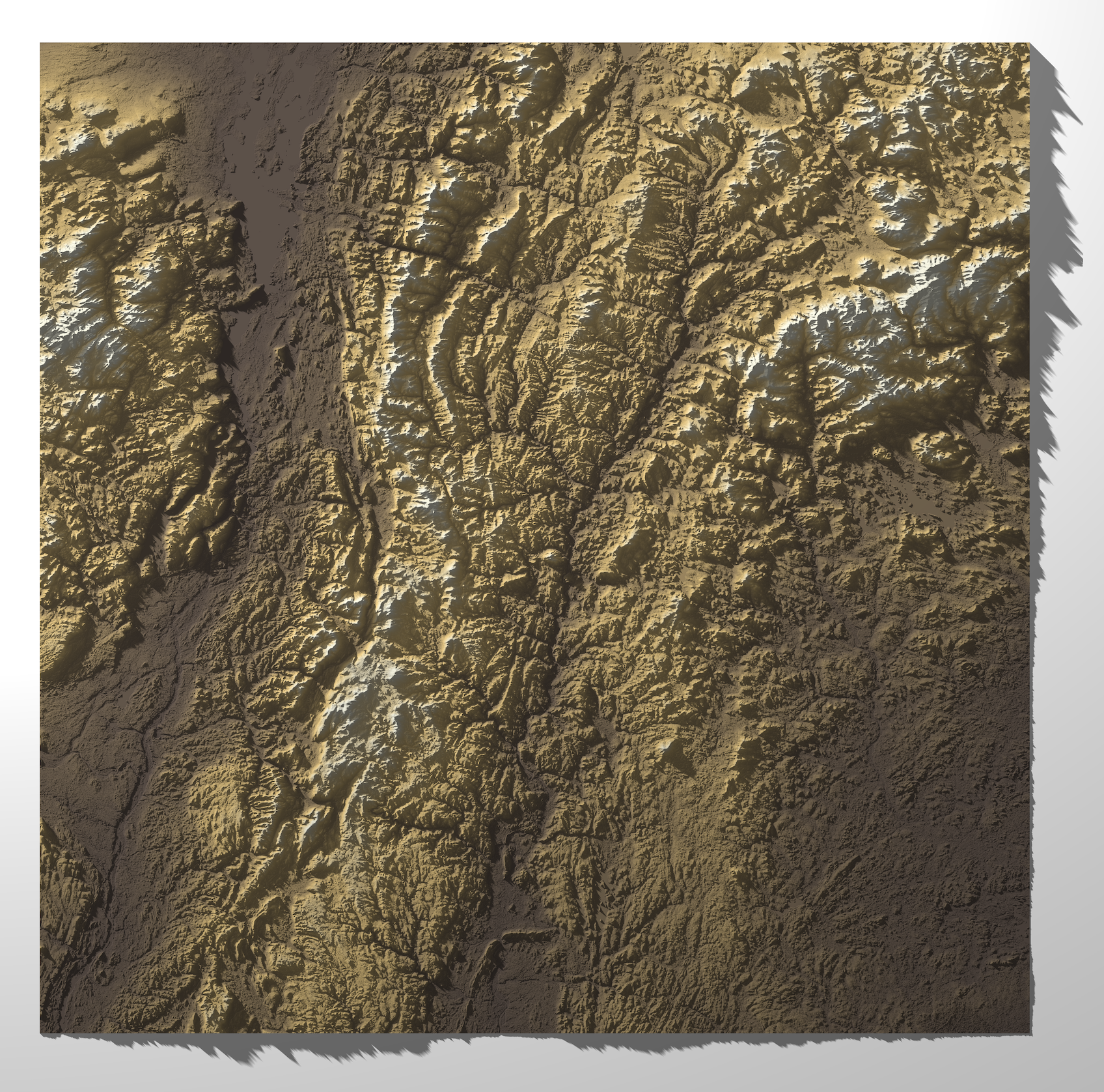
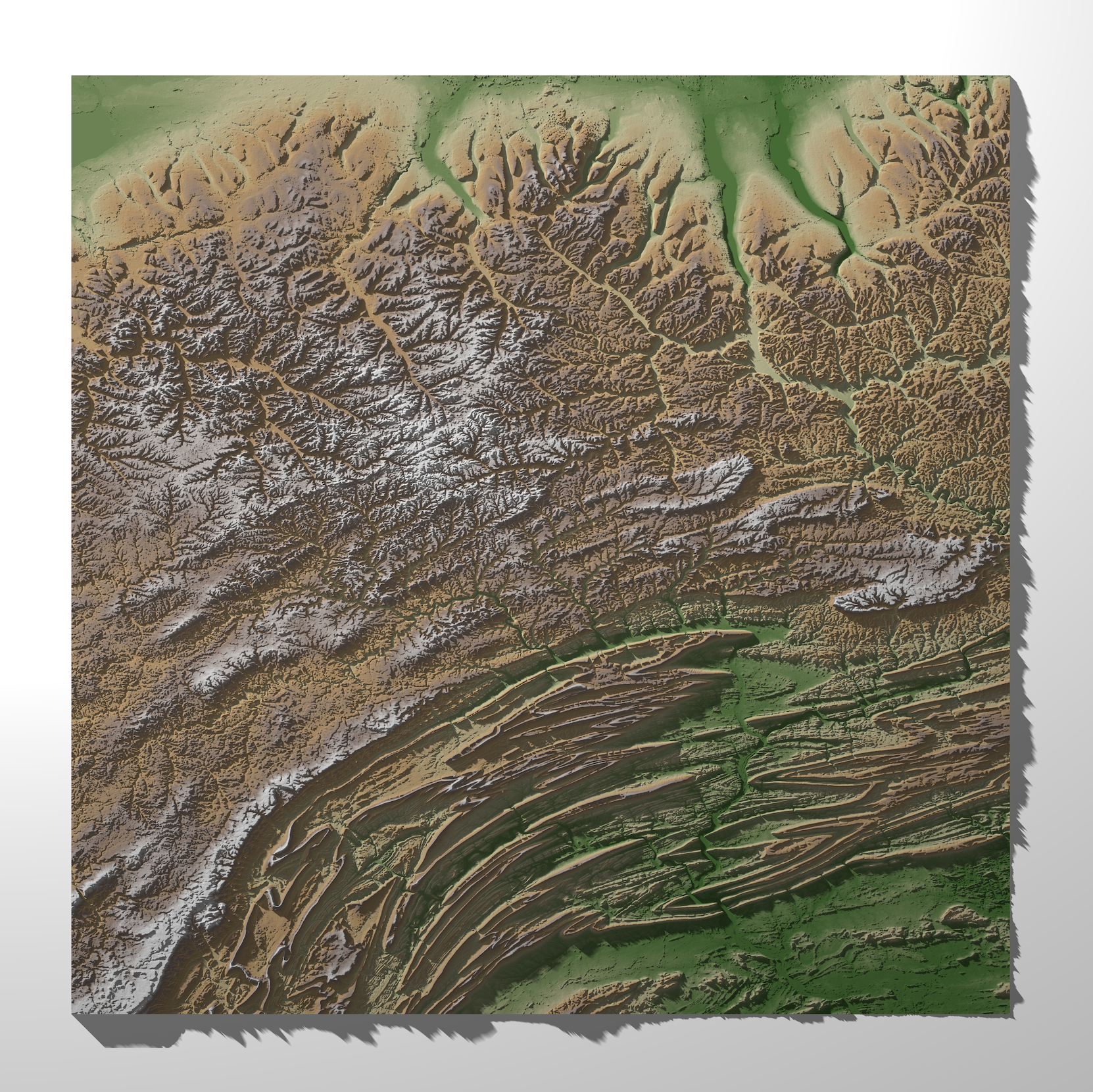
See Also
shadow_image, shadow_animation, time_in_daylight, horizon_angle, hypsometrically_tinted_hillshade
Function Signature
def topo_render(self, dem: Raster, palette: WbPalette = WbPalette.Soft, reverse_palette: bool = False, azimuth: float = 315.0, altitude: float = 30.0, clipping_polygon: Optional[Vector] = None, background_hgt_offset: float = 10.0, background_clr: Tuple[int, int, int, int] = (255, 255, 255, 255), attenuation_parameter: float = 0.3, ambient_light: float = 0.2, z_factor: float = 1.0) -> Raster: ...
topographic_position_animation
License Information
Use of this function requires a license for Whitebox Workflows for Python Professional (WbW-Pro). Please visit www.whiteboxgeo.com to purchase a license.
Description
This tool creates an interactive animation that demonstrates the variation in deviation from mean
elevation (DEV, DevFromMeanElev) as scale increases across a range for an input digital elevation
model (input). DEV is calculated as the difference between the elevation of each grid cell and the
mean elevation of the centering local neighbourhood, normalized by standard deviation and is a measure
of local topographic position. DEV is useful for highlighting locally prominent (either elevated or
low-lying) locations within a landscape. Topographic position animations are extemely useful for
interpreting landscape geomorphic structure across a range of scales.
The set of scales for which DEV is measured (using varying filter sizes) is determined by the three
user-specified parameters, including min_scale, num_steps, and step_nonlinearity. Experience
with DEV scale signatures has shown that it is highly variable at shorter scales and changes more
gradually at broader scales. Therefore, a nonlinear scale sampling interval is used by this tool to
ensure that the scale sampling density is higher for short scale ranges and coarser at longer tested
scales, such that:
ri = rL + (i - rL)p
Where ri is the filter radius for step i, rL is the lower range of filter sizes
(min_scale), and p is the nonlinear scaling factor (step_nonlinearity).
The tool can be run in one of two modes: using regular DEV calculations, or using DEVmax
(max_elevation_deviation), a multiscale version of DEV that outputs the maximum absolute value of
DEV encountered across a range of tested scales. Use the dev_max flag to run the tool in
DEVmax mode.
The output (output) of this tool is an HTML file, containing the interactive GIF animation. Users
are able to zoom and pan around the displayed DEV animation. The DEV images may be rendered in one of several
available palettes (palette) suitable for visualization DEV. The output DEV/DEVmax
animation will also be hillshaded to further enchance topographic interpretation. The user must also
specify the image height (height) in the output file, the time delay (delay, in milliseconds) used
in the GIF animation, and an optional label (label), which will appear in the upper lefthand corner.
Note that the output is simply HTML, CSS, javascript code, and a GIF file, which can be readily embedded
in other documents.
Users should be aware that the outut GIF can be very large in size, depending on the size of the input DEM file. To reduce the file size of the output, it may be desirable to coarsen the input DEM resolution using image resampling (resample).
The following is an example of what the output of this tool looks like. Click the image for an interactive example.
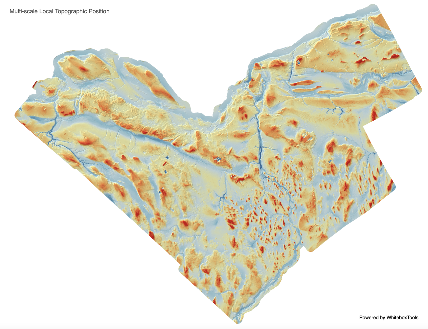
For more information about this tool and example outputs, see this blog on the WhiteboxTools homepage.
See Also
DevFromMeanElev, max_elevation_deviation
Function Signature
def topographic_position_animation(self, dem: Raster, output_html_file: str = "topo_pos.html", palette: WbPalette = WbPalette.Soft, min_scale: int = 1, num_steps: int = 1, step_nonlinearity: float = 1.0, image_height: int = 600, delay: int = 250, label: str = "", use_dev_max: bool = False) -> None: ...
topological_breach_burn
License Information
Use of this function requires a license for Whitebox Workflows for Python Professional (WbW-Pro). Please visit www.whiteboxgeo.com to purchase a license.
Description
This tool performs a specialized form of stream burning, i.e. the practice of forcing the surface flow paths modelled from a digital elevation model (DEM) to match the pathway of a mapped vector stream network. Stream burning is a common flow enforcement technique used to correct surface drainage patterns derived from DEMs. The technique involves adjusting the elevations of grid cells that are coincident with the features of a vector hydrography layer, usually simply by lowering stream cell elevations by a constant offset value. This simple approach is used by the fill_burn tool, which suffers greatly from topological errors resulting from the mismatched scales of the hydrography and DEM data sets. These topological errors, which occur during the rasterization of the stream vector, result in inappropriate stream cell adjacencies (where two stream links appear to be beside one another in the stream raster with no space between) and collisions (where two stream links occupy the same cell in the stream raster). The topological_breach_burn method uses total upstream channel length (TUCL) to prune the vector hydrography layer to a level of detail that matches the raster DEM grid resolution. Network pruning reduces the occurrence of erroneous stream piracy caused by the rasterization of multiple stream links to the same DEM grid cell. The algorithm also restricts flow, during the calculation of the D8 flow pointer raster output, within individual stream reaches, further reducing erroneous stream piracy. In situations where two vector stream features occupy the same grid cell, the new tool ensures that the larger stream, designated by higher TUCL, is given priority. TUCL-based priority minimizes the impact of the topological errors that occur during the stream rasterization process on modelled regional drainage patterns. Lindsay (2016) demonstrated that the topological_breach_burn method produces highly accurate and scale-insensitive drainage patterns and watershed boundaries compared with fill_burn.
The tool requires two input layers, including the DEM (dem) and mapped vector stream network (streams). Note that
these two inputs must share the same map projection. The tool also produces four output rasters, including:
-
A rasterized version of the pruned stream network (
out_streams). Network pruning is based on a TUCL threshold that is calculated as the optimal value that satisfies the combined objectives of maximizing the length of maintained streams and minimizing the number of collisions/adjacencies in the rasterized network. This optimization process is carried out using TUCL and stream length data calculated for each tributary in the network. A tributary connects a channel head and a downstream confluence/outlet in the stream network. Tributaries are often composed of multiple stream links (lengths of streams between upstream-downstream heads/confluences) and can have tributaries of their own. At each confluence in the stream network, the tributary identifier that carries on downstream is associated with the upstream link with the larger TUCL value (a surrogate for stream/drainage area size). The output streams raster shows stream cells remaining after the pruning process along with their unique tributary identifier value. Lower tributary IDs are associated with larger streams, with the lowest valued tributary in a network associated with the main-stem, based on the TUCL criterion for modelling stream size. The main functions of this output are for the user to examine the extent of network pruning used by the tool and to evaluate the network structure described by the tributary IDs. Notice that pruning will be more extensive with a greater mismatch between the scales of the input mapped stream network and the DEM. -
The stream-burned DEM (
out_dem). This DEM will have constantly decreasing elevation values (i.e. breached) along stream tributaries from their channel heads all the way to their eventual outlet points. The tool does not use a constant elevation decrement value. Additionally, all topographic depressions that are located on the hillslopes will be filled; you may pre-process the input DEM with a length-restricted run of the breach_depressions_least_cost tool if you do not wish to fill depressions. This output DEM is probably the least useful of the four output rasters produced by this tool. It is created and output simply because other stream-burning tools produce a burned-in DEM. As indicated above, one of the mechanisms by which this tool improves the topological representation of flow through the rasterized stream network is to ensure that preferential flow path connections are made among stream cells of the same tributary ID and, where there are collisions, to ensure that larger tributaries (lower ID value) is preferred. However, this cannot be represented merely with the elevations contained within this stream-burned DEM. If, for example, you were to run a flow pointer/accumulation operation on the produced DEM, you will not get the exact same outputs as the D8 pointer and flow accumulation rasters produced by this tool, since the D8 tools will not be able to account for the within-tributary flow enforcement used by topological_breach_burn using the elevation values contained within the DEM alone. -
The D8 flow pointer raster (
out_dir). This raster output contains the D8-style pointer values (see the d8_pointer tool for an explanation of pointer value interpretation) and can be used as an input to many of the other hydrological tools in Whitebox. It does capture the topological flow-enforcement within tributaries described above. -
The D8 flow accumulation raster (
out_fa). This raster can be optionally output from the tool if the user specifies a value for this parameter. When specified, the tool will run the standard D8 flow accumulation operation using the flow pointer raster above as input. Note that this raster will be exactly the same as what would be produced should you input the D8 flow pointer produced by this tool to theD8FlowAccumualationtool (thus this output is optional).
The user must lastly specify the snap distance value, in meters. This parameter allows the tool to identify the
linkage between stream segments when their end nodes are not perfectly aligned. One may also choose to run the
repair_stream_vector_topology tool prior to this tool to resolve any misalignment in the input streams vector.
Reference
Lindsay JB. 2016. The practice of DEM stream burning revisited. Earth Surface Processes and Landforms, 41(5): 658–668. DOI: 10.1002/esp.3888
Saunders, W. 1999. Preparation of DEMs for use in environmental modeling analysis, in: ESRI User Conference. pp. 24-30.
See Also
fill_burn, breach_depressions_least_cost, prune_vector_streams, repair_stream_vector_topology, vector_stream_network_analysis
Function Signature
def topological_breach_burn(self, streams: Vector, dem: Raster, snap_distance: float = 0.001) -> Tuple[Raster, Raster, Raster, Raster]: ...
unsphericity
License Information
Use of this function requires a license for Whitebox Workflows for Python Professional (WbW-Pro). Please visit www.whiteboxgeo.com to purchase a license.
Description
This tool calculates the spatial pattern of unsphericity curvature, which describes the degree to which the shape of the topographic surface is nonspherical at a given point (Shary, 1995), from a digital elevation model (DEM). It is calculated as half the difference between the maximal_curvature and the minimal_curvature. Unsphericity has values equal to or greater than zero and is measured in units of m-1. Larger values indicate locations that are less spherical in form.
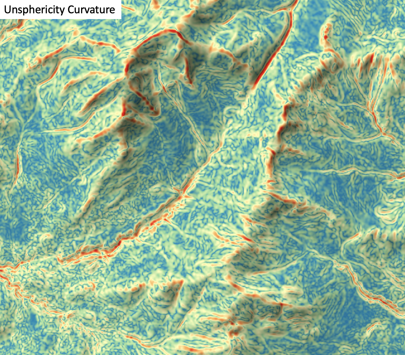
The user must specify the name of the input DEM (dem) and the output raster (output). The
The Z conversion factor (zfactor) is only important when the vertical and horizontal units are not the
same in the DEM. When this is the case, the algorithm will multiply each elevation in the DEM by the
Z Conversion Factor. Curvature values are often very small and as such the user may opt to log-transform
the output raster (log). Transforming the values applies the equation by Shary et al. (2002):
Θ' = sign(Θ) ln(1 + 10n|Θ|)
where Θ is the parameter value and n is dependent on the grid cell size.
For DEMs in projected coordinate systems, the tool uses the 3rd-order bivariate Taylor polynomial method described by Florinsky (2016). Based on a polynomial fit of the elevations within the 5x5 neighbourhood surrounding each cell, this method is considered more robust against outlier elevations (noise) than other methods. For DEMs in geographic coordinate systems (i.e. angular units), the tool uses the 3x3 polynomial fitting method for equal angle grids also described by Florinsky (2016).
References
Florinsky, I. (2016). Digital terrain analysis in soil science and geology. Academic Press.
Florinsky, I. V. (2017). An illustrated introduction to general geomorphometry. Progress in Physical Geography, 41(6), 723-752.
Shary PA (1995) Land surface in gravity points classification by a complete system of curvatures. Mathematical Geology 27: 373–390.
Shary P. A., Sharaya L. S. and Mitusov A. V. (2002) Fundamental quantitative methods of land surface analysis. Geoderma 107: 1–32.
See Also
minimal_curvature, maximal_curvature, mean_curvature, gaussian_curvature, profile_curvature, tangential_curvature
Function Signature
def unsphericity(self, dem: Raster, log_transform: bool = False, z_factor: float = 1.0) -> Raster: ...
vertical_excess_curvature
License Information
Use of this function requires a license for Whitebox Workflows for Python Professional (WbW-Pro). Please visit www.whiteboxgeo.com to purchase a license.
Description
This tool calculates the vertical excess curvature from a digital elevation model (DEM). Vertical excess curvature is the difference of profile (vertical) and minimal curvatures at a location (Shary, 1995). This variable has positive values, zero or greater. Florinsky (2017) states that vertical excess curvature measures the extent to which the bending of a normal section having a common tangent line with a slope line is larger than the minimal bending at a given point of the surface. Vertical excess curvature is measured in units of m-1.
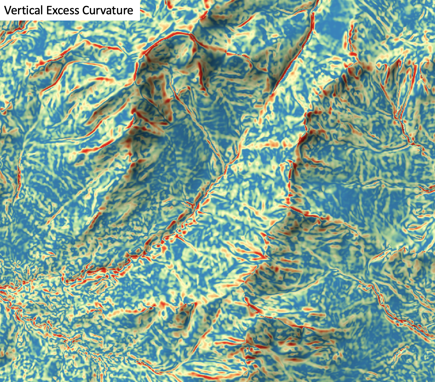
The user must specify the name of the input DEM (dem) and the output raster (output).
The Z conversion factor (zfactor) is only important when the vertical and horizontal units are not the
same in the DEM. When this is the case, the algorithm will multiply each elevation in the DEM by the
Z Conversion Factor. Curvature values are often very small and as such the user may opt to log-transform
the output raster (log). Transforming the values applies the equation by Shary et al. (2002):
Θ' = sign(Θ) ln(1 + 10n|Θ|)
where Θ is the parameter value and n is dependent on the grid cell size.
For DEMs in projected coordinate systems, the tool uses the 3rd-order bivariate Taylor polynomial method described by Florinsky (2016). Based on a polynomial fit of the elevations within the 5x5 neighbourhood surrounding each cell, this method is considered more robust against outlier elevations (noise) than other methods. For DEMs in geographic coordinate systems (i.e. angular units), the tool uses the 3x3 polynomial fitting method for equal angle grids also described by Florinsky (2016).
References
Florinsky, I. (2016). Digital terrain analysis in soil science and geology. Academic Press.
Florinsky, I. V. (2017). An illustrated introduction to general geomorphometry. Progress in Physical Geography, 41(6), 723-752.
Shary PA (1995) Land surface in gravity points classification by a complete system of curvatures. Mathematical Geology 27: 373–390.
Shary P. A., Sharaya L. S. and Mitusov A. V. (2002) Fundamental quantitative methods of land surface analysis. Geoderma 107: 1–32.
See Also
tangential_curvature, profile_curvature, minimal_curvature, maximal_curvature, mean_curvature, gaussian_curvature
Function Signature
def vertical_excess_curvature(self, dem: Raster, log_transform: bool = False, z_factor: float = 1.0) -> Raster: ...
yield_filter
License Information
Use of this function requires a license for Whitebox Workflows for Python Professional (WbW-Pro). Please visit www.whiteboxgeo.com to purchase a license.
Description
This tool can be used to filter the crop yield values associated with point data derived from commerical combine harvester yield monitors. Crop yield data often suffer from high levels of noise do to the nature of how these data are collected. Commercial crop yield monitors on combine haresters are prone to erroneous data for several reasons. Where harvested rows overlap, lower than expected crop yields may be associated with the second overlapping swath because the head of the harvesting equipment is only partially filled. The edges of fields are particularly susceptible to being harvested without a full swath of crop, resulting in anomalous crop yields. The starts of new swaths are also prone to errors, because of the misalignment between the time when the monitor begins recording and the time when grain begins flowing. Sudden changes in harvester speed, either speeing up or slowing down, can also result in anomalous yield measurements.
The yield_filter tool can smooth yield point patterns, particularly accounting for differences among adjacent
swath lines. The user must specify the name of the input points shapefile (input), the name of the yield
attribute (yield_field), the pass number attribute (pass_field_name), the output file (output), the
swatch width (combine head length, width), the threshold value (z_score_threshold), and optionally, minimum
and maximum yield values (min_yield and max_yield). If the input vector does not contain a field indicating
a unique identifier associated with each swath pass for points, users may use the recreate_pass_lines to estimate
swath line structures within the yield points. The threshold value, measured in standardized z-scores
is used by the tool to determine when a point is replaced by the mean value of nearby points in adjacent swaths.
The output vector will contain the smoothed yield data in the attribute table in a field named AVGYIELD.
The following images show before and after examples of applying yield_filter:
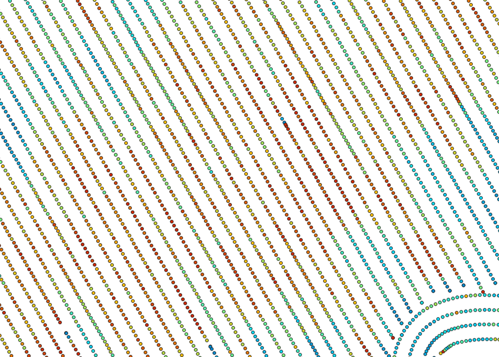
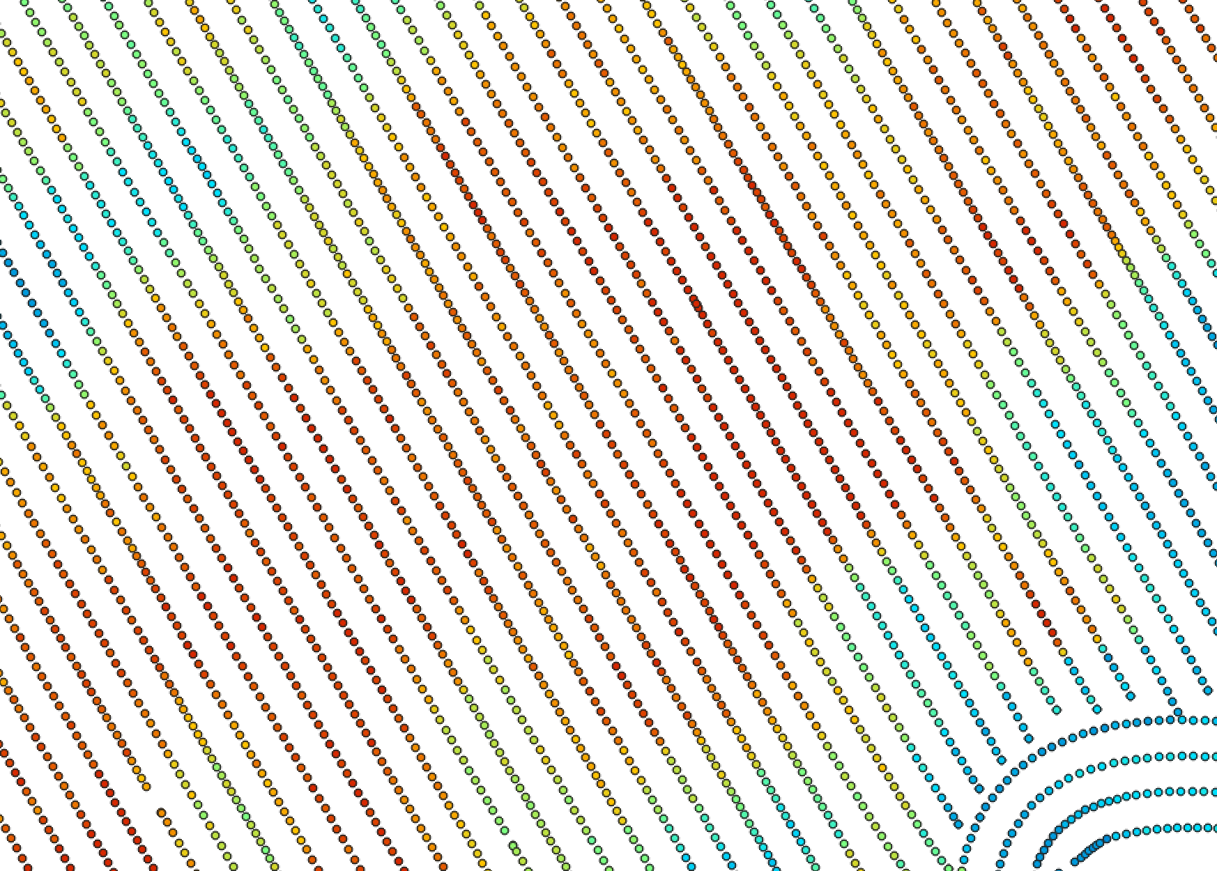
For a video tutorial on how to use the recreate_pass_lines, yield_filter and yield_map tools, see this YouTube video. There is also a blog that describes the usage of this tool on the WhiteboxTools homepage.
See Also
recreate_pass_lines, yield_map, reconcile_multiple_headers, remove_field_edge_points, yield_normalization
Function Signature
def yield_filter(self, input: Vector, yield_field_name: str, pass_field_name: str, swath_width: float = 6.096, z_score_threshold: float = 2.5, min_yield: float = 0.0, max_yield: float = float('inf')) -> Vector: ...
yield_map
License Information
Use of this function requires a license for Whitebox Workflows for Python Professional (WbW-Pro). Please visit www.whiteboxgeo.com to purchase a license.
Description
This tool can be used to create a segmented-vector polygon yield map from a set of harvester points. The user
must specify the name of the input points shapefile (input), the pass number attribute (passFieldName),
the output file (output), the swatch width (combine head length, width), and maximum angular change
in direction (maxChangeInHeading). If the input vector does not contain a field indicating
a unique identifier associated with each swath pass for points, users may use the recreate_pass_lines to estimate
swath line structures within the yield points.
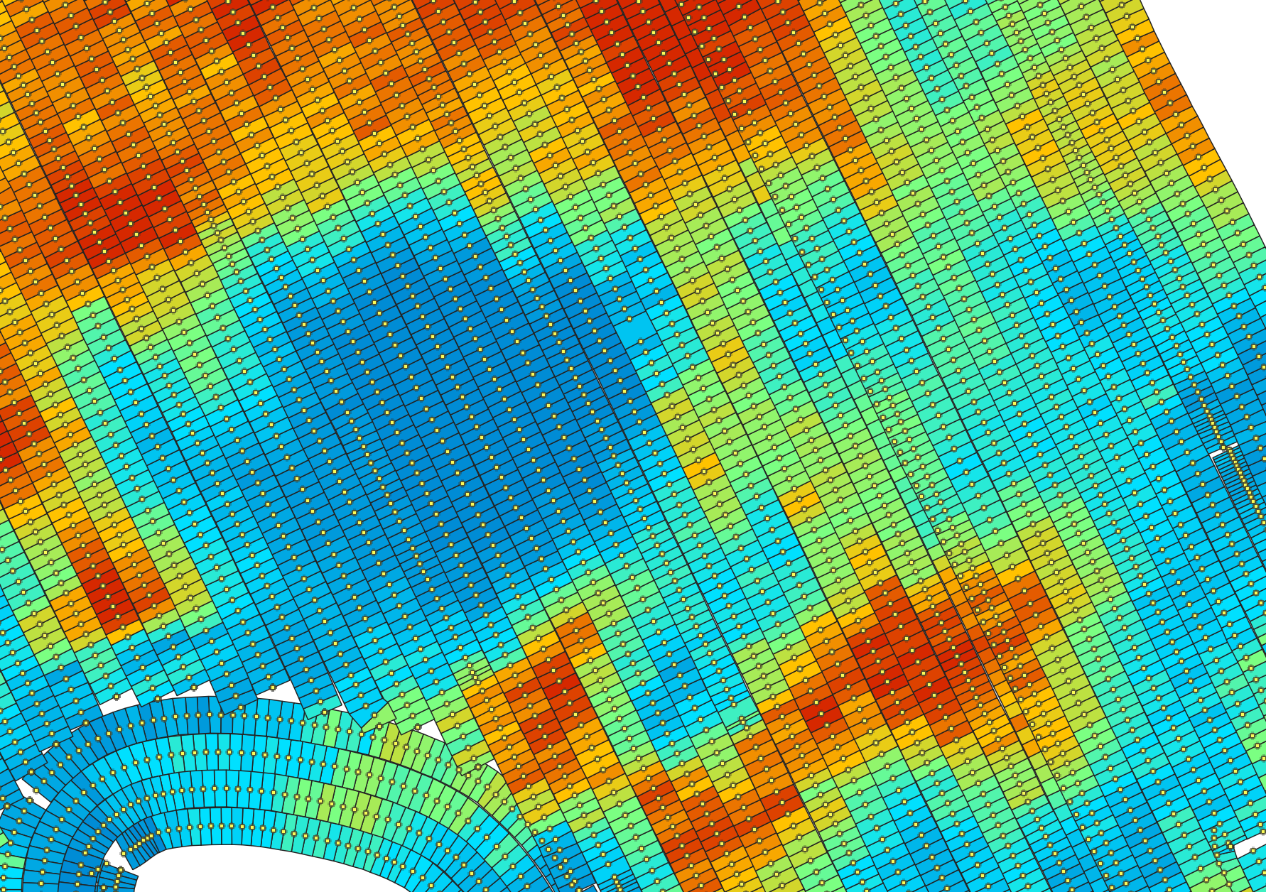
For a video tutorial on how to use the recreate_pass_lines, yield_filter and yield_map tools, see this YouTube video. There is also a blog that describes the usage of this tool on the WhiteboxTools homepage.
See Also
recreate_pass_lines, yield_filter, reconcile_multiple_headers, remove_field_edge_points, yield_normalization
Function Signature
def yield_map(self, input: Vector, pass_field_name: str, swath_width: float = 6.096, max_change_in_heading: float = 25.0) -> Vector: ...
yield_normalization
License Information
Use of this function requires a license for Whitebox Workflows for Python Professional (WbW-Pro). Please visit www.whiteboxgeo.com to purchase a license.
Description
This tool can be used to normalize the crop yield values (yield_field) in a coverage of vector points
(input) derived from a combine harvester for a single agricultural field. Normalization is the process of
modifying the numerical range of a set of values. Normalizing crop yield values is a common pre-processing
procedure prior to analyzing crop data in either a statistical model or machine learning based analysis.
The tool re-scales the crop yield values to a 0.0-1.0 range based on the minimum and maximum values, storing
the rescaled yield data in an attribute field (named NORM_YIELD)) in the output vector file (output).
The user may also specify custom minimum and maximum yield values (min_yield and max_yield); any crop
yield values less than this minimum or larger than the specified maximum will be assigned the boundary values,
and will subsequently define the 0.0-1.0 range.
The user may also optionally choose to standardize (standardize), rather than normalize the data. See
here for
a detailed description of the difference between these two data re-scaling methods. With this
option, the output yield values (stored in the STD_YIELD field of the output vector attribute table) will be
z-scores, based on differences from the mean and scaled by the
standard deviation.
Lastly, the user may optionally specify a search radius (radius), in meters. Without this optional parameter, the
normalization of the data will be based on field-scale values (min/max, or mean/std. dev.). However, when
a radius value larger than zero is specified, the tool will perform a regional analysis based on the points
contained within a local neighbourhood. The radius value should be large enough to ensure that at least
three point measurements are contain within the neighbourhood surrounding each point. Warnings will be issued
for points for which this condition is not met, and their output values will be set to -99.0. When this warning
occurs frequently, you should consider choosing a larger search radius. The following images demonstrate the
difference between field-scale and localized normalization of a sample yield data set.
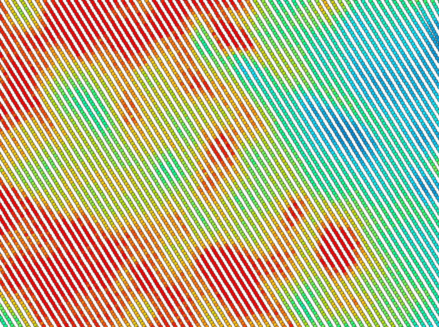
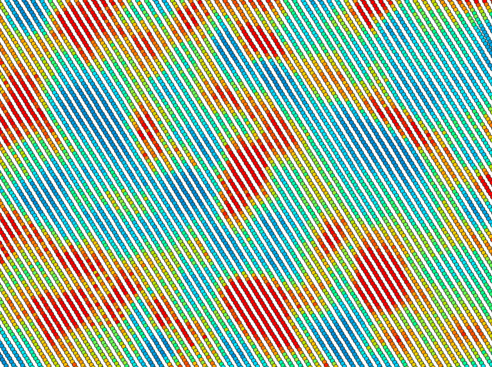
Like many other tools in the Precision Agriculture toolbox, this tool will work with input vector points files in geographic coordinates (i.e. lat/long), although it is preferable to use a projected coordinate system.
See Also
yield_map, yield_filter, recreate_pass_lines, reconcile_multiple_headers, remove_field_edge_points
Function Signature
def yield_normalization(self, input: Vector, yield_field_name: str, radius: float, standardize: bool = False, min_yield: float = 0.0, max_yield: float = float('inf')) -> Vector: ...